-
ACCURACY, PRECISION OF INSTRUMENTS AND ERRORS IN MEASUREMENT
ACCURACY, PRECISION OF INSTRUMENTS AND ERRORS IN MEASUREMENT
Measurement is the foundation of all experimental science and technology.The result of every measurement by any measuring instrument contains some uncertainty.This uncertainty is called error. Every calculated quantity which is based on measured values, also has an error. We shall distinguish between two terms: accuracy and precision.The accuracy of a measurement is a measure of how close the measured value is to the true value of the quantity. Precision tells us to what resolution or limit the quantity is measured.
The accuracy in measurement may depend on several factors, including the limit or the resolution of the measuring instrument. For example, suppose the true value of a certain length is near 3.678 cm.In one experiment,using a measuring instrument of resolution 0.1 cm, the measured value is found to be 3.5 cm, while in another experiment using a measuring device of greater resolution, say 0.01 cm, the length is determined to be 3.38 cm. The first measurement has more accuracy (because it is closer to the true value) but less precision (its resolution is only 0.1 cm), while the second measurement is less accurate but more precise. Thus every measurement is approximate due to errors in measurement. In general, the errors in measurement can be broadly classified as (a) systematic errors and (b) random errors.
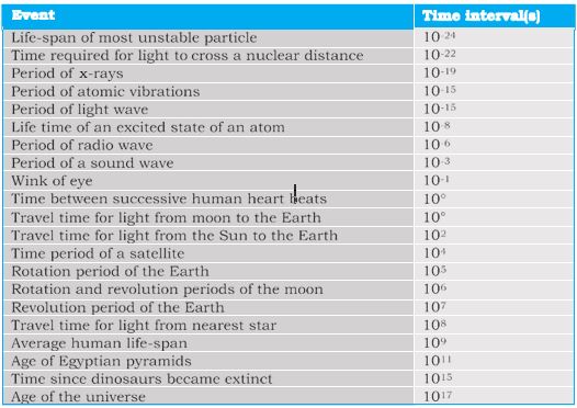
Range and order of time intervals
-
Systematic errors
Systematic Errors
The systematic errors are those errors that tend to be in one direction, either positive or negative.Some of the sources of systematic errors are :
(a).Instrumental errors that arise from the errors due to imperfect design or calibration of the measuring instrument, zero error in the instrument, etc. For example, the temperature graduations of a thermometer may be inadequately calibrated (it may read 104 °C at the boiling point of water at STP whereas it should read 100 °C); in a vernier callipers the zero mark of vernier scale may not coincide with the zero mark of the main scale, or simply an ordinary metre scale may be worn off at one end.
(b)Imperfection in experimental technique or procedure To determine the temperature of a human body, a thermometer placed under the armpit will always give a temperature lower than the actual value of the body temperature.Other external conditions (such as changes in temperature, humidity, wind velocity, etc.) during the experiment may systematically affect the measurement.
(c)Personal errors that arise due to an individual’s bias, lack of proper setting of the apparatus or individual’s carelessness in taking observations without observing proper precautions, etc. For example, if you, by habit, always hold your head a bit too far to the right while reading the position of a needle on the scale, you will introduce an error due to parallax.
Systematic errors can be minimised by improving experimental techniques, selecting better instruments and removing personal bias as far as possible. For a given set-up, these errors may be estimated to a certain extent and the necessary corrections may be applied to the readings.
-
Random Errors
Random Errors
The random errors are those errors, which occur irregularly and hence are random with respect to sign and size.These can arise due to random and unpredictable fluctuations in experimental conditions (e.g. unpredictable fluctuations in temperature,voltage supply, mechanical vibrations of experimental set-ups, etc), personal (unbiased) errors by the observer taking readings, etc. For example, when the same person repeats the same observation, it is very likely that he may get different readings everytime.
-
Least Count Error
Least Count Error
The smallest value that can be measured by the measuring instrument is called its least count.All the readings or measured values are good only up to this value.
The least count error is the error associated with the resolution of the instrument.
For example, a vernier callipers has the least count as 0.01 cm; a spherometer may have a least count of 0.001 cm. Least count error belongs to the category of random errors but within a limited size; it occurs with both systematic and random errors. If we use a metre scale for measurement of length, it may have graduations at 1 mm division scale spacing or interval.
Using instruments of higher precision,improving experimental techniques, etc., we can reduce the least count error. Repeating the observations several times and taking the arithmetic mean of all the observations, the mean value would be very close to the true value of the measured quantity
-
Absolute Error, Relative Error and Percentage Error
Absolute Error, Relative Error and Percentage Error
(a)Suppose the values obtained in several measurements are a1,a2, a3 ...., a .The arithmetic mean of these values is taken as the best possible value of the quantity under the given conditions of measurement as :
\(% MathType!MTEF!2!1!+- % feaagKart1ev2aaatCvAUfeBSjuyZL2yd9gzLbvyNv2CaerbuLwBLn % hiov2DGi1BTfMBaeXatLxBI9gBaerbd9wDYLwzYbItLDharqqtubsr % 4rNCHbGeaGqiVu0Je9sqqrpepC0xbbL8F4rqqrFfpeea0xe9Lq-Jc9 % vqaqpepm0xbba9pwe9Q8fs0-yqaqpepae9pg0FirpepeKkFr0xfr-x % fr-xb9adbaqaaeGaciGaaiaabeqaamaabaabaaGceaqabeaacaWGHb % WaaSbaaSqaaiaad2gacaWGLbGaamyyaiaad6gaaeqaaOGaeyypa0Za % aeWaaeaacaWGHbWaaSbaaSqaaiaaigdaaeqaaOGaey4kaSIaamyyam % aaBaaaleaacaaIYaaabeaakiabgUcaRiaadggadaWgaaWcbaGaaG4m % aaqabaGccqGHRaWkcaGGUaGaaiOlaiaac6cacaGGUaGaaiOlaiaac6 % cacaGGUaGaaiOlaiaac6cacaGGUaGaey4kaSIaamyyamaaBaaaleaa % caWGUbaabeaaaOGaayjkaiaawMcaaiaac+cacaWGUbaabaGaam4Bai % aadkhaaeaacaWGHbWaaSbaaSqaaiaad2gacaWGLbGaamyyaiaad6ga % aeqaaOGaeyypa0ZaaabCaeaacaWGHbWaaSbaaSqaaiaadMgaaeqaaO % Gaai4laiaad6gaaSqaaiaadMgacqGH9aqpcaaIXaaabaGaamOBaaqd % cqGHris5aaaaaa!626D! \begin{array}{l} {a_{mean}} = \left( {{a_1} + {a_2} + {a_3} + .......... + {a_n}} \right)/n\\ or\\ {a_{mean}} = \sum\limits_{i = 1}^n {{a_i}/n} \end{array}\)
This is because, as explained earlier, it is reasonable to suppose that individual measurements are as likely to overestimate as to underestimate the true value of the quantity.
The magnitude of the difference between the individual measurement and the true value of the quantity is called the absolute error of the measurement. This is denoted by \(% MathType!MTEF!2!1!+- % feaagKart1ev2aaatCvAUfeBSjuyZL2yd9gzLbvyNv2CaerbuLwBLn % hiov2DGi1BTfMBaeXatLxBI9gBaerbd9wDYLwzYbItLDharqqtubsr % 4rNCHbGeaGqiVu0Je9sqqrpepC0xbbL8F4rqqrFfpeea0xe9Lq-Jc9 % vqaqpepm0xbba9pwe9Q8fs0-yqaqpepae9pg0FirpepeKkFr0xfr-x % fr-xb9adbaqaaeGaciGaaiaabeqaamaabaabaaGcbaWaaqWaaeaacq % GHuoarcaWGHbaacaGLhWUaayjcSdaaaa!3B65! \left| {\Delta a} \right|\) In absence of any other method of knowing true value, we considered arithmatic mean as the true value. Then the errors in the individual measurement values from the true value, are
\(\Delta\)a1=a1-amean,
\(\Delta\)a2=a2-amean
\(\Delta\)an=an-amean
The \(\Delta\)a calculated above may be positive in certain cases and negative in some other cases.But absolute error \(% MathType!MTEF!2!1!+- % feaagKart1ev2aaatCvAUfeBSjuyZL2yd9gzLbvyNv2CaerbuLwBLn % hiov2DGi1BTfMBaeXatLxBI9gBaerbd9wDYLwzYbItLDharqqtubsr % 4rNCHbGeaGqiVu0Je9sqqrpepC0xbbL8F4rqqrFfpeea0xe9Lq-Jc9 % vqaqpepm0xbba9pwe9Q8fs0-yqaqpepae9pg0FirpepeKkFr0xfr-x % fr-xb9adbaqaaeGaciGaaiaabeqaamaabaabaaGcbaWaaqWaaeaacq % GHuoarcaWGHbaacaGLhWUaayjcSdaaaa!3B65! \left| {\Delta a} \right|\) will always be positive.
(b)The arithmetic mean of all the absolute errors is taken as the final or mean absolute error of the value of the physical quantity a. It is
represented by \(\Delta\)amean.
Thus,
\(% MathType!MTEF!2!1!+- % feaagKart1ev2aaatCvAUfeBSjuyZL2yd9gzLbvyNv2CaerbuLwBLn % hiov2DGi1BTfMBaeXatLxBI9gBaerbd9wDYLwzYbItLDharqqtubsr % 4rNCHbGeaGqiVu0Je9sqqrpepC0xbbL8F4rqqrFfpeea0xe9Lq-Jc9 % vqaqpepm0xbba9pwe9Q8fs0-yqaqpepae9pg0FirpepeKkFr0xfr-x % fr-xb9adbaqaaeGaciGaaiaabeqaamaabaabaaGceaqabeaacqGHuo % arcaWGHbWaaSbaaSqaaiaad2gacaWGLbGaamyyaiaad2gaaeqaaOGa % eyypa0ZaaeWaaeaadaabdaqaaiabgs5aejaadggadaWgaaWcbaGaaG % ymaaqabaaakiaawEa7caGLiWoacqGHRaWkdaabdaqaaiabgs5aejaa % dggadaWgaaWcbaGaaGOmaaqabaaakiaawEa7caGLiWoadaabdaqaai % abgs5aejaadggadaWgaaWcbaGaaG4maaqabaaakiaawEa7caGLiWoa % cqGHRaWkcaGGUaGaaiOlaiaac6cacaGGUaGaaiOlaiaac6cacaGGUa % GaaiOlaiabgUcaRmaaemaabaGaeyiLdqKaamyyamaaBaaaleaacaWG % UbaabeaaaOGaay5bSlaawIa7aaGaayjkaiaawMcaaiaac+cacaWGUb % aabaGaeyypa0ZaaabCaeaadaabdaqaaiabgs5aejaadggadaWgaaWc % baGaamyAaaqabaaakiaawEa7caGLiWoacaGGVaGaamOBaaWcbaGaam % yAaiabg2da9iaaigdaaeaacaWGUbaaniabggHiLdaaaaa!717D! \begin{array}{l} \Delta {a_{meam}} = \left( {\left| {\Delta {a_1}} \right| + \left| {\Delta {a_2}} \right|\left| {\Delta {a_3}} \right| + ........ + \left| {\Delta {a_n}} \right|} \right)/n\\ = \sum\limits_{i = 1}^n {\left| {\Delta {a_i}} \right|/n} \end{array}\)
If we do a single measurement, the value we get may be in the range amean \(% MathType!MTEF!2!1!+- % feaagKart1ev2aaatCvAUfeBSjuyZL2yd9gzLbvyNv2CaerbuLwBLn % hiov2DGi1BTfMBaeXatLxBI9gBaerbd9wDYLwzYbItLDharqqtubsr % 4rNCHbGeaGqiVu0Je9sqqrpepC0xbbL8F4rqqrFfpeea0xe9Lq-Jc9 % vqaqpepm0xbba9pwe9Q8fs0-yqaqpepae9pg0FirpepeKkFr0xfr-x % fr-xb9adbaqaaeGaciGaaiaabeqaamaabaabaaGcbaGaeyySaeRaey % iLdqeaaa!394B! \pm \Delta \) amean
i.e; a=amean\(% MathType!MTEF!2!1!+- % feaagKart1ev2aaatCvAUfeBSjuyZL2yd9gzLbvyNv2CaerbuLwBLn % hiov2DGi1BTfMBaeXatLxBI9gBaerbd9wDYLwzYbItLDharqqtubsr % 4rNCHbGeaGqiVu0Je9sqqrpepC0xbbL8F4rqqrFfpeea0xe9Lq-Jc9 % vqaqpepm0xbba9pwe9Q8fs0-yqaqpepae9pg0FirpepeKkFr0xfr-x % fr-xb9adbaqaaeGaciGaaiaabeqaamaabaabaaGcbaGaeyySaeRaey % iLdqeaaa!394B! \pm \Delta \)amean
or
\(% MathType!MTEF!2!1!+- % feaagKart1ev2aaatCvAUfeBSjuyZL2yd9gzLbvyNv2CaerbuLwBLn % hiov2DGi1BTfMBaeXatLxBI9gBaerbd9wDYLwzYbItLDharqqtubsr % 4rNCHbGeaGqiVu0Je9sqqrpepC0xbbL8F4rqqrFfpeea0xe9Lq-Jc9 % vqaqpepm0xbba9pwe9Q8fs0-yqaqpepae9pg0FirpepeKkFr0xfr-x % fr-xb9adbaqaaeGaciGaaiaabeqaamaabaabaaGcbaGaamyyamaaBa % aaleaacaWGTbGaamyzaiaadggacaWGUbaabeaakiabgkHiTiabgs5a % ejaadggadaWgaaWcbaGaamyBaiaadwgacaWGHbGaamOBaaqabaGccq % GHKjYOcaWGHbGaeyizImQaamyyamaaBaaaleaacaWGTbGaamyzaiaa % dggacaWGUbaabeaakiabgUcaRiabgs5aejaadggadaWgaaWcbaGaam % yBaiaadwgacaWGHbGaamOBaaqabaaaaa!521D! {a_{mean}} - \Delta {a_{mean}} \le a \le {a_{mean}} + \Delta {a_{mean}}\)
This implies that any measurement of the physical quantity a is likely to lie between (a+\(\Delta\)a)and(a-\(\Delta\)a)
(c)Instead of the absolute error,we often use (\(% MathType!MTEF!2!1!+- % feaagKart1ev2aaatCvAUfeBSjuyZL2yd9gzLbvyNv2CaerbuLwBLn % hiov2DGi1BTfMBaeXatLxBI9gBaerbd9wDYLwzYbItLDharqqtubsr % 4rNCHbGeaGqiVu0Je9sqqrpepC0xbbL8F4rqqrFfpeea0xe9Lq-Jc9 % vqaqpepm0xbba9pwe9Q8fs0-yqaqpepae9pg0FirpepeKkFr0xfr-x % fr-xb9adbaqaaeGaciGaaiaabeqaamaabaabaaGcbaGaeqiTdqgaaa!379B! \delta \)a).The relative error is the ratio of the mean absolute error \(\Delta\)a to the mean value a of the quantity measured.
Relative error =\(% MathType!MTEF!2!1!+- % feaagKart1ev2aaatCvAUfeBSjuyZL2yd9gzLbvyNv2CaerbuLwBLn % hiov2DGi1BTfMBaeXatLxBI9gBaerbd9wDYLwzYbItLDharqqtubsr % 4rNCHbGeaGqiVu0Je9sqqrpepC0xbbL8F4rqqrFfpeea0xe9Lq-Jc9 % vqaqpepm0xbba9pwe9Q8fs0-yqaqpepae9pg0FirpepeKkFr0xfr-x % fr-xb9adbaqaaeGaciGaaiaabeqaamaabaabaaGcbaGaeyiLdqKaam % yyamaaBaaaleaacaWGTbGaamyzaiaadggacaWGUbaabeaakiaac+ca % caWGHbWaaSbaaSqaaiaad2gacaWGLbGaamyyaiaad6gaaeqaaaaa!41A8! \Delta {a_{mean}}/{a_{mean}}\)
When the relative error is expressed in per cent, it is called the percentage error ( \(% MathType!MTEF!2!1!+- % feaagKart1ev2aaatCvAUfeBSjuyZL2yd9gzLbvyNv2CaerbuLwBLn % hiov2DGi1BTfMBaeXatLxBI9gBaerbd9wDYLwzYbItLDharqqtubsr % 4rNCHbGeaGqiVu0Je9sqqrpepC0xbbL8F4rqqrFfpeea0xe9Lq-Jc9 % vqaqpepm0xbba9pwe9Q8fs0-yqaqpepae9pg0FirpepeKkFr0xfr-x % fr-xb9adbaqaaeGaciGaaiaabeqaamaabaabaaGcbaGaeqiTdqgaaa!379B! \delta \)a)
Thus, Percentage error
\(% MathType!MTEF!2!1!+- % feaagKart1ev2aaatCvAUfeBSjuyZL2yd9gzLbvyNv2CaerbuLwBLn % hiov2DGi1BTfMBaeXatLxBI9gBaerbd9wDYLwzYbItLDharqqtubsr % 4rNCHbGeaGqiVu0Je9sqqrpepC0xbbL8F4rqqrFfpeea0xe9Lq-Jc9 % vqaqpepm0xbba9pwe9Q8fs0-yqaqpepae9pg0FirpepeKkFr0xfr-x % fr-xb9adbaqaaeGaciGaaiaabeqaamaabaabaaGcbaGaeqiTdqMaam % yyaiabg2da9maabmaabaGaeyiLdqKaamyyamaaBaaaleaacaWGTbGa % amyzaiaadggacaWGUbGaai4laaqabaGccaWGHbWaaSbaaSqaaiaad2 % gacaWGLbGaamyyaiaad6gaaeqaaaGccaGLOaGaayzkaaGaey41aqRa % aGymaiaaicdacaaIWaGaaiyjaaaa!4BBB! \delta a = \left( {\Delta {a_{mean/}}{a_{mean}}} \right) \times 100\% \)
EXAMPLE 6
Two clocks are being tested against a standard clock located in a national laboratory. At 12:00:00 noon by the standard clock, the readings of the two clocks are :
If you are doing an experiment that requires precision time interval measurements, which of the two clocks will you prefer ?
Answer:-
The range of variation over the seven days of observations is 162 s for clock 1, and 31 s for clock 2. The average reading of clock 1 is much closer to the standard time than the average reading of clock 2. The important point is that a clock’s zero error is not as significant for precision work as its variation, because a ‘zero-error’ can always be easily corrected. Hence clock 2 is to be preferred to clock 1.
EXAMPLE 7
We measure the period of oscillation of a simple pendulum.In successive measurements, the readings turn out to be 2.63 s, 2.56 s, 2.42 s, 2.71s and 2.80 s. Calculate the absolute errors, relative error or percentage error.
Answer:-
The mean period of oscillation of the pendulum
\(% MathType!MTEF!2!1!+- % feaagKart1ev2aaatCvAUfeBSjuyZL2yd9gzLbvyNv2CaerbuLwBLn % hiov2DGi1BTfMBaeXatLxBI9gBaerbd9wDYLwzYbItLDharqqtubsr % 4rNCHbGeaGqiVu0Je9sqqrpepC0xbbL8F4rqqrFfpeea0xe9Lq-Jc9 % vqaqpepm0xbba9pwe9Q8fs0-yqaqpepae9pg0FirpepeKkFr0xfr-x % fr-xb9adbaqaaeGaciGaaiaabeqaamaabaabaaGceaqabeaacaWGub % Gaeyypa0ZaaSaaaeaadaqadaqaaiaaikdacaGGUaGaaGOnaiaaioda % cqGHRaWkcaaIYaGaaiOlaiaaiwdacaaI2aGaey4kaSIaaGOmaiaac6 % cacaaI0aGaaGOmaiabgUcaRiaaikdacaGGUaGaaG4naiaaigdacqGH % RaWkcaaIYaGaaiOlaiaaiIdacaaIWaaacaGLOaGaayzkaaGaam4Caa % qaaiaaiwdaaaaabaGaeyypa0ZaaSaaaeaacaaIXaGaaG4maiaac6ca % caaIXaGaaGOmaaqaaiaaiwdaaaGaam4Caaaaaa!53B6! \begin{array}{l} T = \frac{{\left( {2.63 + 2.56 + 2.42 + 2.71 + 2.80} \right)s}}{5}\\ = \frac{{13.12}}{5}s \end{array}\)
=2.624 s
=2.62 s
As the periods are measured to a resolution of 0.01 s, all times are to the second decimal; it is proper to put this mean period also to the second decimal.
The errors in the measurements are 2.63 s – 2.62 s = 0.01 s
2.56 s – 2.62 s = – 0.06 s
2.42 s – 2.62 s = – 0.20 s
2.71 s – 2.62 s = 0.09 s
2.80 s – 2.62 s = 0.18 s
Note that the errors have the same units as the quantity to be measured.The arithmetic mean of all the absolute errors (for arithmetic mean, we take only the magnitudes) is
\(% MathType!MTEF!2!1!+- % feaagKart1ev2aaatCvAUfeBSjuyZL2yd9gzLbvyNv2CaerbuLwBLn % hiov2DGi1BTfMBaeXatLxBI9gBaerbd9wDYLwzYbItLDharqqtubsr % 4rNCHbGeaGqiVu0Je9sqqrpepC0xbbL8F4rqqrFfpeea0xe9Lq-Jc9 % vqaqpepm0xbba9pwe9Q8fs0-yqaqpepae9pg0FirpepeKkFr0xfr-x % fr-xb9adbaqaaeGaciGaaiaabeqaamaabaabaaGcbaGaeyiLdqKaam % ivamaaBaaaleaacaWGTbGaamyzaiaadggacaWGUbaabeaaaaa!3C17! \Delta {T_{mean}}\)= [(0.01+ 0.06+0.20+0.09+0.18)s]/5
=0.54 s/5
=0.11 s
That means, the period of oscillation of the simple pendulum is (2.62 ± 0.11) s i.e. it lies between (2.62 + 0.11) s and (2.62 – 0.11) s or between 2.73 s and 2.51 s. As the arithmetic mean of all the absolute errors is 0.11 s, there is already an error in the tenth of a second. Hence there is no point in giving the period to a hundredth. A more correct way will be to write
T=2.6±0.1 s
Note that the last numeral 6 is unreliable, since it may be anything between 5 and 7.We indicate this by saying that the measurement has two significant figures.In this case, the two significant figures are 2, which is reliable and 6, which has an error associated with it. You will learn more about the significant figures in section 2.7.
For this example, the relative error or the percentage error is
\(% MathType!MTEF!2!1!+- % feaagKart1ev2aaatCvAUfeBSjuyZL2yd9gzLbvyNv2CaerbuLwBLn % hiov2DGi1BTfMBaeXatLxBI9gBaerbd9wDYLwzYbItLDharqqtubsr % 4rNCHbGeaGqiVu0Je9sqqrpepC0xbbL8F4rqqrFfpeea0xe9Lq-Jc9 % vqaqpepm0xbba9pwe9Q8fs0-yqaqpepae9pg0FirpepeKkFr0xfr-x % fr-xb9adbaqaaeGaciGaaiaabeqaamaabaabaaGcbaGaeqiTdqMaam % yyaiabg2da9maalaaabaGaaGimaiaac6cacaaIXaaabaGaaGOmaiaa % c6cacaaI2aaaaiabgEna0kaaigdacaaIWaGaaGimaiabg2da9iaais % dacaGGLaaaaa!449F! \delta a = \frac{{0.1}}{{2.6}} \times 100 = 4\% \)
-
Combination of Errors
Combination of Errors
If we do an experiment involving several measurements, we must know how the errors in all the measurements combine. For example,mass density is obtained by deviding mass by the volume of the substance. If we have errors in the measurement of mass and of the sizes or dimensions, we must know what the error will be in the density of the substance. To make such estimates, we should learn how errors combine in various mathematical operations. For this, we use the following procedure.
(a)Error of a sum or a different
Suppose two physical quantities A and B have measured values A ± \(\Delta\)A, B ± \(\Delta\)B respectively where \(\Delta\)A and \(\Delta\)B are their absolute errors. We wish to find the error \(\Delta\)Z in the sum Z=A+B.
We have by addition, Z \(\Delta\) \(\Delta\)Z= (A ± \(\Delta\)A) + (B ± \(\Delta\)B).
The maximum possible error in Z
\(\Delta\)Z ± \(\Delta\)A + \(\Delta\)B
For the difference Z = A – B, we have
Z ± \(\Delta\) Z = (A ± \(\Delta\)A) – (B ± \(\Delta\)B)
= (A – B) ± \(\Delta\)A ± \(\Delta\)B
or, ± \(\Delta\)Z = ± \(\Delta\)A ±\(\Delta\)B
The maximum value of the error \(\Delta\)Z is again
\(\Delta\)A + \(\Delta\)B.
Hence the rule : When two quantities are added or subtracted, the absolute error in the final result is the sum of the absolute errors in the individual quantities.EXAMPLE 8
The temperatures of two bodies measured by a thermometer are t1 = 20 0C ± 0.5 0C and t2 = 500C ± 0.5 0C.Calculate the temperature difference and the error theirin.
ANSWER
\(% MathType!MTEF!2!1!+- % feaagKart1ev2aaatCvAUfeBSjuyZL2yd9gzLbvyNv2CaerbuLwBLn % hiov2DGi1BTfMBaeXatLxBI9gBaerbd9wDYLwzYbItLDharqqtubsr % 4rNCHbGeaGqiVu0Je9sqqrpepC0xbbL8F4rqqrFfpeea0xe9Lq-Jc9 % vqaqpepm0xbba9pwe9Q8fs0-yqaqpepae9pg0FirpepeKkFr0xfr-x % fr-xb9adbaqaaeGaciGaaiaabeqaamaabaabaaGceaqabeaaceWG0b % GbauaacqGH9aqpcaWG0bWaaSbaaSqaaiaaikdaaeqaaOGaeyOeI0Ia % amiDamaaBaaaleaacaaIXaaabeaakiabg2da9maabmaabaGaaGynai % aaicdadaahaaWcbeqaaiaaicdaaaGccaWGdbGaeyySaeRaaGimaiaa % c6cacaaI1aWaaWbaaSqabeaacaaIWaaaaOGaam4qaaGaayjkaiaawM % caaiabgkHiTmaabmaabaGaaGOmaiaaicdadaahaaWcbeqaaiaaicda % aaGccaWGdbGaeyySaeRaaGimaiaac6cacaaI1aWaaWbaaSqabeaaca % aIWaaaaOGaam4qaaGaayjkaiaawMcaaaqaaiqadshagaqbaiabg2da % 9iaaiodacaaIWaWaaWbaaSqabeaacaaIWaaaaOGaam4qaiabgglaXk % aaigdadaahaaWcbeqaaiaaicdaaaGccaWGdbaaaaa!5D71! \begin{array}{l} t' = {t_2} - {t_1} = \left( {{{50}^0}C \pm {{0.5}^0}C} \right) - \left( {{{20}^0}C \pm {{0.5}^0}C} \right)\\ t' = {30^0}C \pm {1^0}C \end{array}\)
(b)Error of a product or a quotient
Suppose Z = AB and the measured values of A
and B are A ± \(\Delta\)A and B ± \(\Delta\)B. Then
Z ± \(\Delta\)Z = (A ± \(\Delta\)A) (B ± \(\Delta\)B)
= AB ± B \(\Delta\)A ± A \(\Delta\)B ± \(\Delta\)A \(\Delta\)B.
Dividing LHS by Z and RHS by AB we have, 1±(\(\Delta\)Z/Z) = 1 ± (\(\Delta\)A/A) ± (\(\Delta\)B/B) ± (\(\Delta\)A/A)(\(\Delta\)B/B).
Since \(\Delta\)A and \(\Delta\)B are small, we shall ignore their product.
Hence the maximum relative error
\(\Delta\)Z/ Z = (\(\Delta\)A/A) + (\(\Delta\)B/B).
You can easily verify that this is true for division also.
Hence the rule :When two quantities are multiplied or divided, the relative error in the result is the sum of the relative errors in the multipliers.
EXAMPLES 9
The resistance R = V/I where V = (100 ± 5)V and I = (10 ± 0.2)A. Find the percentage error in R.
ANSWER:-
The percentage error in V is 5% and in I it is 2%. The total error in R would therefore be 5% + 2% = 7%.
EXAMPLE 10
Two resistors of resistances R1 = 100 ± 3 ohm and R2 = 200 ± 4 ohm are connected (a) in series, (b) in parallel. Find the equivalent resistance of the (a) series combination, (b) parallel combination. Use for (a) the relation R = R1 + R2, and for (b)\(% MathType!MTEF!2!1!+- % feaagKart1ev2aaatCvAUfeBSjuyZL2yd9gzLbvyNv2CaerbuLwBLn % hiov2DGi1BTfMBaeXatLxBI9gBaerbd9wDYLwzYbItLDharqqtubsr % 4rNCHbGeaGqiVu0Je9sqqrpepC0xbbL8F4rqqrFfpeea0xe9Lq-Jc9 % vqaqpepm0xbba9pwe9Q8fs0-yqaqpepae9pg0FirpepeKkFr0xfr-x % fr-xb9adbaqaaeGaciGaaiaabeqaamaabaabaaGcbaWaaSaaaeaaca % aIXaaabaGabmOuayaafaaaaiabg2da9maalaaabaGaaGymaaqaaiaa % dkfadaWgaaWcbaGaaGymaaqabaaaaOGaey4kaSYaaSaaaeaacaaIXa % aabaGaamOuamaaBaaaleaacaaIYaaabeaaaaGccaaMc8UaaGPaVlaa % ykW7caWGHbGaamOBaiaadsgacaaMc8UaaGPaVlaaykW7daWcaaqaai % abgs5aejqadkfagaqbaaqaaiqadkfagaqbamaaCaaaleqabaGaaGOm % aaaaaaGccqGH9aqpdaWcaaqaaiabgs5aejaadkfadaWgaaWcbaGaaG % ymaaqabaaakeaacaWGsbWaa0baaSqaaiaaigdaaeaacaaIYaaaaaaa % kiabgUcaRmaalaaabaGaeyiLdqKaamOuamaaBaaaleaacaaIYaaabe % aaaOqaaiaadkfadaqhaaWcbaGaaGOmaaqaaiaaikdaaaaaaaaa!5C4F! \frac{1}{{R'}} = \frac{1}{{{R_1}}} + \frac{1}{{{R_2}}}\,\,\,and\,\,\,\frac{{\Delta R'}}{{{{R'}^2}}} = \frac{{\Delta {R_1}}}{{R_1^2}} + \frac{{\Delta {R_2}}}{{R_2^2}}\)
ANSWER
(a)The equivalent resistance of series combination
R = R1 + R2 = (100 ± 3) ohm + (200 ± 4) ohm
= 300 ± 7 ohm.
(b)The equivalent resistance of parallel combination
\(% MathType!MTEF!2!1!+- % feaagKart1ev2aaatCvAUfeBSjuyZL2yd9gzLbvyNv2CaerbuLwBLn % hiov2DGi1BTfMBaeXatLxBI9gBaerbd9wDYLwzYbItLDharqqtubsr % 4rNCHbGeaGqiVu0Je9sqqrpepC0xbbL8F4rqqrFfpeea0xe9Lq-Jc9 % vqaqpepm0xbba9pwe9Q8fs0-yqaqpepae9pg0FirpepeKkFr0xfr-x % fr-xb9adbaqaaeGaciGaaiaabeqaamaabaabaaGcbaGabmOuayaafa % Gaeyypa0ZaaSaaaeaacaWGsbWaaSbaaSqaaiaaigdaaeqaaOGaamOu % amaaBaaaleaacaaIYaaabeaaaOqaaiaadkfadaWgaaWcbaGaaGymaa % qabaGccqGHRaWkcaWGsbWaaSbaaSqaaiaaikdaaeqaaaaakiabg2da % 9maalaaabaGaaGOmaiaaicdacaaIWaaabaGaaG4maaaacqGH9aqpca % aI2aGaaGOnaiaac6cacaaI3aGaam4BaiaadIgacaWGTbaaaa!4AC2! R' = \frac{{{R_1}{R_2}}}{{{R_1} + {R_2}}} = \frac{{200}}{3} = 66.7ohm\)
Then from,\(% MathType!MTEF!2!1!+- % feaagKart1ev2aaatCvAUfeBSjuyZL2yd9gzLbvyNv2CaerbuLwBLn % hiov2DGi1BTfMBaeXatLxBI9gBaerbd9wDYLwzYbItLDharqqtubsr % 4rNCHbGeaGqiVu0Je9sqqrpepC0xbbL8F4rqqrFfpeea0xe9Lq-Jc9 % vqaqpepm0xbba9pwe9Q8fs0-yqaqpepae9pg0FirpepeKkFr0xfr-x % fr-xb9adbaqaaeGaciGaaiaabeqaamaabaabaaGcbaWaaSaaaeaaca % aIXaaabaGabmOuayaafaaaaiabg2da9maalaaabaGaaGymaaqaaiaa % dkfadaWgaaWcbaGaaGymaaqabaaaaOGaey4kaSYaaSaaaeaacaaIXa % aabaGaamOuamaaBaaaleaacaaIYaaabeaaaaaaaa!3EA9! \frac{1}{{R'}} = \frac{1}{{{R_1}}} + \frac{1}{{{R_2}}}\)
we get,
\(% MathType!MTEF!2!1!+- % feaagKart1ev2aaatCvAUfeBSjuyZL2yd9gzLbvyNv2CaerbuLwBLn % hiov2DGi1BTfMBaeXatLxBI9gBaerbd9wDYLwzYbItLDharqqtubsr % 4rNCHbGeaGqiVu0Je9sqqrpepC0xbbL8F4rqqrFfpeea0xe9Lq-Jc9 % vqaqpepm0xbba9pwe9Q8fs0-yqaqpepae9pg0FirpepeKkFr0xfr-x % fr-xb9adbaqaaeGaciGaaiaabeqaamaabaabaaGceaqabeaadaWcaa % qaaiabgs5aejqadkfagaqbaaqaaiqadkfagaqbamaaCaaaleqabaGa % aGOmaaaaaaGccqGH9aqpdaWcaaqaaiabgs5aejaadkfadaWgaaWcba % GaaGymaaqabaaakeaacaWGsbWaa0baaSqaaiaaigdaaeaacaaIYaaa % aaaakiabgUcaRmaalaaabaGaeyiLdqKaamOuamaaBaaaleaacaaIYa % aabeaaaOqaaiaadkfadaqhaaWcbaGaaGOmaaqaaiaaikdaaaaaaaGc % baGaeyiLdqKabmOuayaafaGaeyypa0ZaaeWaaeaaceWGsbGbauaada % ahaaWcbeqaaiaaikdaaaaakiaawIcacaGLPaaadaWcaaqaaiabgs5a % ejaadkfadaWgaaWcbaGaaGymaaqabaaakeaacaWGsbWaa0baaSqaai % aaigdaaeaacaaIYaaaaaaakiabgUcaRmaabmaabaGabmOuayaafaWa % aWbaaSqabeaacaaIYaaaaaGccaGLOaGaayzkaaWaaSaaaeaacqGHuo % arcaWGsbWaaSbaaSqaaiaaikdaaeqaaaGcbaGaamOuamaaDaaaleaa % caaIYaaabaGaaGOmaaaaaaaakeaacqGH9aqpdaqadaqaamaalaaaba % GaaGOnaiaaiAdacaGGUaGaaG4naaqaaiaaigdacaaIWaGaaGimaaaa % aiaawIcacaGLPaaadaahaaWcbeqaaiaaikdaaaGccaaIZaGaey4kaS % YaaeWaaeaadaWcaaqaaiaaiAdacaaI2aGaaiOlaiaaiEdaaeaacaaI % YaGaaGimaiaaicdaaaaacaGLOaGaayzkaaWaaWbaaSqabeaacaaIYa % aaaOGaaGinaaqaaiabg2da9iaaigdacaGGUaGaaGioaaaaaa!7410! \begin{array}{l} \frac{{\Delta R'}}{{{{R'}^2}}} = \frac{{\Delta {R_1}}}{{R_1^2}} + \frac{{\Delta {R_2}}}{{R_2^2}}\\ \Delta R' = \left( {{{R'}^2}} \right)\frac{{\Delta {R_1}}}{{R_1^2}} + \left( {{{R'}^2}} \right)\frac{{\Delta {R_2}}}{{R_2^2}}\\ = {\left( {\frac{{66.7}}{{100}}} \right)^2}3 + {\left( {\frac{{66.7}}{{200}}} \right)^2}4\\ = 1.8 \end{array}\)
Then,\(% MathType!MTEF!2!1!+- % feaagKart1ev2aaatCvAUfeBSjuyZL2yd9gzLbvyNv2CaerbuLwBLn % hiov2DGi1BTfMBaeXatLxBI9gBaerbd9wDYLwzYbItLDharqqtubsr % 4rNCHbGeaGqiVu0Je9sqqrpepC0xbbL8F4rqqrFfpeea0xe9Lq-Jc9 % vqaqpepm0xbba9pwe9Q8fs0-yqaqpepae9pg0FirpepeKkFr0xfr-x % fr-xb9adbaqaaeGaciGaaiaabeqaamaabaabaaGcbaGabmOuayaafa % aaaa!36D9! {R'}\) 66.7 \(% MathType!MTEF!2!1!+- % feaagKart1ev2aaatCvAUfeBSjuyZL2yd9gzLbvyNv2CaerbuLwBLn % hiov2DGi1BTfMBaeXatLxBI9gBaerbd9wDYLwzYbItLDharqqtubsr % 4rNCHbGeaGqiVu0Je9sqqrpepC0xbbL8F4rqqrFfpeea0xe9Lq-Jc9 % vqaqpepm0xbba9pwe9Q8fs0-yqaqpepae9pg0FirpepeKkFr0xfr-x % fr-xb9adbaqaaeGaciGaaiaabeqaamaabaabaaGcbaGaeyySaelaaa!37E4! \pm \)1.8 ohmR
(Here, \(\Delta\)R is expresed as 1.8 instead of 2 to keep in confirmity with the rules of significant figures.)
(c)Error in case of a measured quantity raised to a power
Suppose Z = A2,
Then,
\(\Delta\)Z/Z = (\(\Delta\)A/A) + (\(\Delta\)A/A) = 2 (\(\Delta\)A/A).
Hence, the relative error in A2 is two times the error in A.
In general, if Z = Ap Bq/Cr
Then,
\(\Delta\)Z/Z = p (\(\Delta\)A/A) + q (\(\Delta\)B/B) + r (\(\Delta\)C/C).
Hence the rule : The relative error in a physical quantity raised to the power k is the k times the relative error in the individual quantity.EXAMPLE 11
Find the relative error in Z, if Z = A4B1/3/CD3/2.
ANSWER
The relative error in Z is \(\Delta\)Z/Z = 4(\(\Delta\)A/A) +(1/3) (\(\Delta\)B/B) + (\(\Delta\)C/C) + (3/2) (\(\Delta\)D/D).
EXAMPLE 12
The period of oscillation of a simple pendulum is T \(\sqrt{L/g}=2\pi\).Measured value of L is 20.0 cm known to 1 mm accuracy and time for 100 oscillations of the pendulum is found to be 90 s using a wrist watch of 1 s resolution. What is the accuracy in the determination of g ?
ANSWER
g=4\(\pi\)L/T2
\(% MathType!MTEF!2!1!+- % feaagKart1ev2aaatCvAUfeBSjuyZL2yd9gzLbvyNv2CaerbuLwBLn % hiov2DGi1BTfMBaeXatLxBI9gBaerbd9wDYLwzYbItLDharqqtubsr % 4rNCHbGeaGqiVu0Je9sqqrpepC0xbbL8F4rqqrFfpeea0xe9Lq-Jc9 % vqaqpepm0xbba9pwe9Q8fs0-yqaqpepae9pg0FirpepeKkFr0xfr-x % fr-xb9adbaqaaeGaciGaaiaabeqaamaabaabaaGcbaGaamisaiaadw % gacaWGYbGaamyzaiaacYcacaWGubGaeyypa0ZaaSaaaeaacaWG0baa % baGaamOBaaaacaWGHbGaamOBaiaadsgacqGHuoarcaWGubGaeyypa0 % ZaaSaaaeaacqGHuoarcaWG0baabaGaamOBaaaacaGGUaGaamivaiaa % dIgacaWGLbGaamOCaiaadwgacaWGMbGaam4BaiaadkhacaWGLbGaey % ypa0ZaaSaaaeaacqGHuoarcaWG0baabaGaamivaaaacqGH9aqpdaWc % aaqaaiabgs5aejaadshaaeaacaWG0baaaaaa!5945! Here,T = \frac{t}{n}and\Delta T = \frac{{\Delta t}}{n}.Therefore = \frac{{\Delta t}}{T} = \frac{{\Delta t}}{t}\)
The errors in both L and t are the least count errors.Therefore
\(% MathType!MTEF!2!1!+- % feaagKart1ev2aaatCvAUfeBSjuyZL2yd9gzLbvyNv2CaerbuLwBLn % hiov2DGi1BTfMBaeXatLxBI9gBaerbd9wDYLwzYbItLDharqqtubsr % 4rNCHbGeaGqiVu0Je9sqqrpepC0xbbL8F4rqqrFfpeea0xe9Lq-Jc9 % vqaqpepm0xbba9pwe9Q8fs0-yqaqpepae9pg0FirpepeKkFr0xfr-x % fr-xb9adbaqaaeGaciGaaiaabeqaamaabaabaaGceaqabeaadaqada % qaaiabgs5aejaadEgacaGGVaGaam4zaaGaayjkaiaawMcaaiabg2da % 9maabmaabaGaeyiLdqKaamitaiaac+cacaWGmbaacaGLOaGaayzkaa % Gaey4kaSIaaGOmamaabmaabaGaeyiLdqKaamivaiaac+cacaWGubaa % caGLOaGaayzkaaaabaGaeyypa0ZaaSaaaeaacaaIWaGaaiOlaiaaig % daaeaacaaIYaGaaGimaiaac6cacaaIWaaaaiabgUcaRiaaikdadaqa % daqaamaalaaabaGaaGymaaqaaiaaiMdacaaIWaaaaaGaayjkaiaawM % caaiabg2da9iaaicdacaGGUaGaaGimaiaaikdacaaI3aaaaaa!58ED! \begin{array}{l} \left( {\Delta g/g} \right) = \left( {\Delta L/L} \right) + 2\left( {\Delta T/T} \right)\\ = \frac{{0.1}}{{20.0}} + 2\left( {\frac{1}{{90}}} \right) = 0.027 \end{array}\)
Thus, the percentage error in g is
\(% MathType!MTEF!2!1!+- % feaagKart1ev2aaatCvAUfeBSjuyZL2yd9gzLbvyNv2CaerbuLwBLn % hiov2DGi1BTfMBaeXatLxBI9gBaerbd9wDYLwzYbItLDharqqtubsr % 4rNCHbGeaGqiVu0Je9sqqrpepC0xbbL8F4rqqrFfpeea0xe9Lq-Jc9 % vqaqpepm0xbba9pwe9Q8fs0-yqaqpepae9pg0FirpepeKkFr0xfr-x % fr-xb9adbaqaaeGaciGaaiaabeqaamaabaabaaGcbaGaaGymaiaaic % dacaaIWaWaaeWaaeaacqGHuoarcaWGNbGaai4laiaadEgaaiaawIca % caGLPaaacqGH9aqpcaaIXaGaaGimaiaaicdadaqadaqaaiabgs5aej % aadYeacaGGVaGaamitaaGaayjkaiaawMcaaiabgUcaRiaaikdacqGH % xdaTcaaIXaGaaGimaiaaicdadaqadaqaaiabgs5aejaadsfacaGGVa % GaamivaaGaayjkaiaawMcaaaaa!5153! 100\left( {\Delta g/g} \right) = 100\left( {\Delta L/L} \right) + 2 \times 100\left( {\Delta T/T} \right)\)=3%