-
Position Vector and Displacement
Position Vector and Displacement
In this section we shall see how to describe motion in two dimensions using vectors.
The position vector r of a particle P located in a plane with reference to the origin of an x-y reference frame (Fig. 4.12) is given by \(% MathType!MTEF!2!1!+- % feaagKart1ev2aaatCvAUfeBSjuyZL2yd9gzLbvyNv2CaerbuLwBLn % hiov2DGi1BTfMBaeXatLxBI9gBaerbd9wDYLwzYbItLDharqqtubsr % 4rNCHbGeaGqiVu0Je9sqqrpepC0xbbL8F4rqqrFfpeea0xe9Lq-Jc9 % vqaqpepm0xbba9pwe9Q8fs0-yqaqpepae9pg0FirpepeKkFr0xfr-x % fr-xb9adbaqaaeGaciGaaiaabeqaamaabaabaaGcbaGaamOCaiabg2 % da9iaadIhaceWGPbGbaKaacqGHRaWkcaWG5bGabmOAayaajaaaaa!3CCD! r = x\hat i + y\hat j\).
where x and y are components of r along x-, and y- axes or simply they are the coordinates of the object.
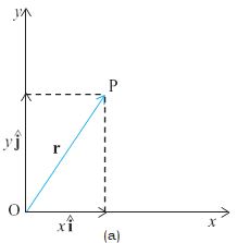
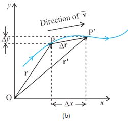
fig.4.12.a) Position vector r. (b) Displacement \(\Delta\)r and average velocity v of a particle
Suppose a particle moves along the curve shown by the thick line and is at P at time t and \(% MathType!MTEF!2!1!+- % feaagKart1ev2aaatCvAUfeBSjuyZL2yd9gzLbvyNv2CaerbuLwBLn % hiov2DGi1BTfMBaeXatLxBI9gBaerbd9wDYLwzYbItLDharqqtubsr % 4rNCHbGeaGqiVu0Je9sqqrpepC0xbbL8F4rqqrFfpeea0xe9Lq-Jc9 % vqaqpepm0xbba9pwe9Q8fs0-yqaqpepae9pg0FirpepeKkFr0xfr-x % fr-xb9adbaqaaeGaciGaaiaabeqaamaabaabaaGcbaGabmiuayaafa % aaaa!36D7! P'\) at time \(% MathType!MTEF!2!1!+- % feaagKart1ev2aaatCvAUfeBSjuyZL2yd9gzLbvyNv2CaerbuLwBLn % hiov2DGi1BTfMBaeXatLxBI9gBaerbd9wDYLwzYbItLDharqqtubsr % 4rNCHbGeaGqiVu0Je9sqqrpepC0xbbL8F4rqqrFfpeea0xe9Lq-Jc9 % vqaqpepm0xbba9pwe9Q8fs0-yqaqpepae9pg0FirpepeKkFr0xfr-x % fr-xb9adbaqaaeGaciGaaiaabeqaamaabaabaaGcbaGabmiDayaafa % aaaa!36FB! t'\) [Fig. 4.12(b)]. Then, the displacement is :
\(% MathType!MTEF!2!1!+- % feaagKart1ev2aaatCvAUfeBSjuyZL2yd9gzLbvyNv2CaerbuLwBLn % hiov2DGi1BTfMBaeXatLxBI9gBaerbd9wDYLwzYbItLDharqqtubsr % 4rNCHbGeaGqiVu0Je9sqqrpepC0xbbL8F4rqqrFfpeea0xe9Lq-Jc9 % vqaqpepm0xbba9pwe9Q8fs0-yqaqpepae9pg0FirpepeKkFr0xfr-x % fr-xb9adbaqaaeGaciGaaiaabeqaamaabaabaaGcbaGaeyiLdqKaam % OCaiabg2da9iqadkhagaqbaiabgkHiTiaadkhaaaa!3C41! \Delta r = r' - r\)
and is directed from P to\(% MathType!MTEF!2!1!+- % feaagKart1ev2aaatCvAUfeBSjuyZL2yd9gzLbvyNv2CaerbuLwBLn % hiov2DGi1BTfMBaeXatLxBI9gBaerbd9wDYLwzYbItLDharqqtubsr % 4rNCHbGeaGqiVu0Je9sqqrpepC0xbbL8F4rqqrFfpeea0xe9Lq-Jc9 % vqaqpepm0xbba9pwe9Q8fs0-yqaqpepae9pg0FirpepeKkFr0xfr-x % fr-xb9adbaqaaeGaciGaaiaabeqaamaabaabaaGcbaGabmiuayaafa % aaaa!36D7! P'\).
We can write Eq. (4.25) in a component form:
\(% MathType!MTEF!2!1!+- % feaagKart1ev2aaatCvAUfeBSjuyZL2yd9gzLbvyNv2CaerbuLwBLn % hiov2DGi1BTfMBaeXatLxBI9gBaerbd9wDYLwzYbItLDharqqtubsr % 4rNCHbGeaGqiVu0Je9sqqrpepC0xbbL8F4rqqrFfpeea0xe9Lq-Jc9 % vqaqpepm0xbba9pwe9Q8fs0-yqaqpepae9pg0FirpepeKkFr0xfr-x % fr-xb9adbaqaaeGaciGaaiaabeqaamaabaabaaGceaqabeaacqGHuo % arcaWGYbGaeyypa0ZaaeWaaeaaceWG4bGbauaaceWGPbGbaKaacqGH % RaWkceWG5bGbauaaceWGQbGbaKaaaiaawIcacaGLPaaacqGHsislda % qadaqaaiaadIhaceWGPbGbaKaacqGHRaWkcaWG5bGabmOAayaajaaa % caGLOaGaayzkaaaabaGaeyypa0JabmyAayaajaGaeyiLdqKaamiEai % abgUcaRiqadQgagaqcaiabgs5aejaadMhaaeaacaWG3bGaamiAaiaa % dwgacaWGYbGaamyzaiabgs5aejaadIhacqGH9aqpceWG4bGbauaacq % GHsislcaWG4bGaaiilaiabgs5aejaadMhacqGH9aqpceWG5bGbauaa % cqGHsislcaWG5baaaaa!61FC! \begin{array}{l} \Delta r = \left( {x'\hat i + y'\hat j} \right) - \left( {x\hat i + y\hat j} \right)\\ = \hat i\Delta x + \hat j\Delta y\\ where\Delta x = x' - x,\Delta y = y' - y \end{array}\)
-
Velocity
Velocity
 The average velocity \(% MathType!MTEF!2!1!+-
% feaagKart1ev2aaatCvAUfeBSjuyZL2yd9gzLbvyNv2CaerbuLwBLn
% hiov2DGi1BTfMBaeXatLxBI9gBaerbd9wDYLwzYbItLDharqqtubsr
% 4rNCHbGeaGqiVu0Je9sqqrpepC0xbbL8F4rqqrFfpeea0xe9Lq-Jc9
% vqaqpepm0xbba9pwe9Q8fs0-yqaqpepae9pg0FirpepeKkFr0xfr-x
% fr-xb9adbaqaaeGaciGaaiaabeqaamaabaabaaGcbaWaaeWaaeaada
% qdaaqaaiaadAhaaaaacaGLOaGaayzkaaaaaa!388B!
\left( {\overline v } \right)\) of an object is the ratio of the displacement and the corresponding time interval :
The average velocity \(% MathType!MTEF!2!1!+-
% feaagKart1ev2aaatCvAUfeBSjuyZL2yd9gzLbvyNv2CaerbuLwBLn
% hiov2DGi1BTfMBaeXatLxBI9gBaerbd9wDYLwzYbItLDharqqtubsr
% 4rNCHbGeaGqiVu0Je9sqqrpepC0xbbL8F4rqqrFfpeea0xe9Lq-Jc9
% vqaqpepm0xbba9pwe9Q8fs0-yqaqpepae9pg0FirpepeKkFr0xfr-x
% fr-xb9adbaqaaeGaciGaaiaabeqaamaabaabaaGcbaWaaeWaaeaada
% qdaaqaaiaadAhaaaaacaGLOaGaayzkaaaaaa!388B!
\left( {\overline v } \right)\) of an object is the ratio of the displacement and the corresponding time interval :\(% MathType!MTEF!2!1!+- % feaagKart1ev2aaatCvAUfeBSjuyZL2yd9gzLbvyNv2CaerbuLwBLn % hiov2DGi1BTfMBaeXatLxBI9gBaerbd9wDYLwzYbItLDharqqtubsr % 4rNCHbGeaGqiVu0Je9sqqrpepC0xbbL8F4rqqrFfpeea0xe9Lq-Jc9 % vqaqpepm0xbba9pwe9Q8fs0-yqaqpepae9pg0FirpepeKkFr0xfr-x % fr-xb9adbaqaaeGaciGaaiaabeqaamaabaabaaGceaqabeaadaqdaa % qaaiaadAhaaaGaeyypa0ZaaSaaaeaacqGHuoarcaWGYbaabaGaeyiL % dqKaamiDaaaacqGH9aqpdaWcaaqaaiabgs5aejaadIhaceWGPbGbaK % aacqGHRaWkcqGHuoarcaWG5bGabmOAayaajaaabaGaeyiLdqKaamiD % aaaacqGH9aqpceWGPbGbaKaadaWcaaqaaiabgs5aejaadIhaaeaacq % GHuoarcaWG0baaaiabgUcaRiqadQgagaqcamaalaaabaGaeyiLdqKa % amyEaaqaaiabgs5aejaadshaaaaabaGaam4BaiaadkhacaGGSaWaa0 % aaaeaacaWG2baaaiabg2da9maanaaabaGaamODaaaadaWgaaWcbaGa % amiEaaqabaGcceWGPbGbaKaacqGHRaWkdaqdaaqaaiaadAhaaaWaaS % baaSqaaiaadMhaaeqaaOGabmOAayaajaaaaaa!6194! \begin{array}{l} \overline v = \frac{{\Delta r}}{{\Delta t}} = \frac{{\Delta x\hat i + \Delta y\hat j}}{{\Delta t}} = \hat i\frac{{\Delta x}}{{\Delta t}} + \hat j\frac{{\Delta y}}{{\Delta t}}\\ or,\overline v = {\overline v _x}\hat i + {\overline v _y}\hat j \end{array}\)
Since \(% MathType!MTEF!2!1!+- % feaagKart1ev2aaatCvAUfeBSjuyZL2yd9gzLbvyNv2CaerbuLwBLn % hiov2DGi1BTfMBaeXatLxBI9gBaerbd9wDYLwzYbItLDharqqtubsr % 4rNCHbGeaGqiVu0Je9sqqrpepC0xbbL8F4rqqrFfpeea0xe9Lq-Jc9 % vqaqpepm0xbba9pwe9Q8fs0-yqaqpepae9pg0FirpepeKkFr0xfr-x % fr-xb9adbaqaaeGaciGaaiaabeqaamaabaabaaGcbaWaa0aaaeaaca % WG2baaaiabg2da9maalaaabaGaeyiLdqKaamOCaaqaaiabgs5aejaa % dshaaaaaaa!3CD6! \overline v = \frac{{\Delta r}}{{\Delta t}}\),the direction of the average velocity is the same as that of \(\Delta\)r (Fig. 4.12). The velocity (instantaneous velocity) is given by the limiting value of the average velocity as the time interval approaches zero :
\(% MathType!MTEF!2!1!+- % feaagKart1ev2aaatCvAUfeBSjuyZL2yd9gzLbvyNv2CaerbuLwBLn % hiov2DGi1BTfMBaeXatLxBI9gBaerbd9wDYLwzYbItLDharqqtubsr % 4rNCHbGeaGqiVu0Je9sqqrpepC0xbbL8F4rqqrFfpeea0xe9Lq-Jc9 % vqaqpepm0xbba9pwe9Q8fs0-yqaqpepae9pg0FirpepeKkFr0xfr-x % fr-xb9adbaqaaeGaciGaaiaabeqaamaabaabaaGcbaGaamODaiabg2 % da9maaxacabaGaeyiLdqKaamiDaiabgkziUkaaicdaaSqabeaaciGG % SbGaaiyAaiaac2gaaaGcdaWcaaqaaiabgs5aejaadkhaaeaacqGHuo % arcaWG0baaaiabg2da9maalaaabaGaamizaiaadkhaaeaacaWGKbGa % amiDaaaaaaa!49C7! v = \mathop {\Delta t \to 0}\limits^{\lim } \frac{{\Delta r}}{{\Delta t}} = \frac{{dr}}{{dt}}\)
The meaning of the limiting process can be easily understood with the help of Fig 4.13(a) to (d). In these figures, the thick line represents the path of an object, which is at P at time t. P1, P2 and P3 represent the positions of the object after times \(\Delta\)t1 ,\(\Delta\)t2, and\(\Delta\)t3. \(\Delta\)r1, \(\Delta\)r2, and \(\Delta\)r3 are the displacements of the object in times \(\Delta\)t1, \(\Delta\)t2, and \(\Delta\)t3, respectively.
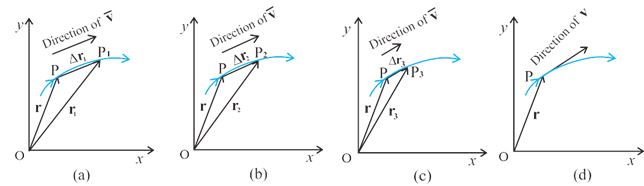
fig.4.13. As the time interval \(\Delta\)t approaches zero, the average velocity approaches the velocity v.The direction of v is parallel to the line tangent to the path.
The direction of the average velocity v is shown in figures (a), (b) and (c) for three decreasing values of \(\Delta\)t, i.e. \(\Delta\)t 1,\(\Delta\)t2, and \(\Delta\)t3,\(% MathType!MTEF!2!1!+- % feaagKart1ev2aaatCvAUfeBSjuyZL2yd9gzLbvyNv2CaerbuLwBLn % hiov2DGi1BTfMBaeXatLxBI9gBaerbd9wDYLwzYbItLDharqqtubsr % 4rNCHbGeaGqiVu0Je9sqqrpepC0xbbL8F4rqqrFfpeea0xe9Lq-Jc9 % vqaqpepm0xbba9pwe9Q8fs0-yqaqpepae9pg0FirpepeKkFr0xfr-x % fr-xb9adbaqaaeGaciGaaiaabeqaamaabaabaaGcbaWaaeWaaeaacq % GHuoarcaWG0bWaaSbaaSqaaiaaigdaaeqaaOGaeyOpa4JaeyiLdqKa % amiDamaaBaaaleaacaaIYaaabeaakiabg6da+iabgs5aejaadshada % WgaaWcbaGaaG4maaqabaaakiaawIcacaGLPaaacaGGUaGaamyqaiaa % dohacaaMc8UaaGPaVlabgs5aejaadshacqGHsgIRcaaIWaGaaiilai % abgs5aejaadkhacqGHsgIRcaaIWaaaaa!53C7! \left( {\Delta {t_1} > \Delta {t_2} > \Delta {t_3}} \right).As\,\,\Delta t \to 0,\Delta r \to 0\) and is along the tangent to the path [Fig. 4.13(d)]. Therefore, the direction of velocity at any point on the path of an object is tangential to the path at that point and is in the direction of motion.
We can express v in a component form :
\(% MathType!MTEF!2!1!+- % feaagKart1ev2aaatCvAUfeBSjuyZL2yd9gzLbvyNv2CaerbuLwBLn % hiov2DGi1BTfMBaeXatLxBI9gBaerbd9wDYLwzYbItLDharqqtubsr % 4rNCHbGeaGqiVu0Je9sqqrpepC0xbbL8F4rqqrFfpeea0xe9Lq-Jc9 % vqaqpepm0xbba9pwe9Q8fs0-yqaqpepae9pg0FirpepeKkFr0xfr-x % fr-xb9adbaqaaeGaciGaaiaabeqaamaabaabaaGceaqabeaacaWG2b % Gaeyypa0ZaaSaaaeaacaWGKbGaamOCaaqaaiaadsgacaWG0baaaaqa % aiabg2da9maaxacabaGaeyiLdqKaamiDaiabgkziUkaaicdaaSqabe % aaciGGSbGaaiyAaiaac2gaaaGcdaqadaqaamaalaaabaGaeyiLdqKa % amiEaaqaaiabgs5aejaadshaaaGabmyAayaajaGaey4kaSYaaSaaae % aacqGHuoarcaWG5baabaGaeyiLdqKaamiDaaaaceWGQbGbaKaaaiaa % wIcacaGLPaaaaeaacqGH9aqpceWGPbGbaKaadaWfGaqaaiabgs5aej % aadshacqGHsgIRcaaIWaaaleqabaGaciiBaiaacMgacaGGTbaaaOWa % aSaaaeaacqGHuoarcaWG4baabaGaeyiLdqKaamiDaaaacqGHRaWkce % WGQbGbaKaadaWfGaqaaiabgs5aejaadshacqGHsgIRcaaIWaaaleqa % baGaciiBaiaacMgacaGGTbaaaOWaaSaaaeaacqGHuoarcaWG5baaba % GaeyiLdqKaamiDaaaaaeaacaWGpbGaamOCaiaacYcacaWG2bGaeyyp % a0JabmyAayaajaWaaSaaaeaacaWGKbGaamiEaaqaaiaadsgacaWG0b % aaaiabgUcaRiqadQgagaqcamaalaaabaGaamizaiaadMhaaeaacaWG % KbGaamiDaaaacqGH9aqpcaWG2bWaaSbaaSqaaiaadIhaaeqaaOGabm % yAayaajaGaey4kaSIaamODamaaBaaaleaacaWG5baabeaakiqadQga % gaqcaiaac6caaeaacaWG3bGaamiAaiaadwgacaWGYbGaamyzaiaadA % hadaWgaaWcbaGaamiEaaqabaGccqGH9aqpdaWcaaqaaiabgs5aejaa % dIhaaeaacqGHuoarcaWG0baaaiaacYcacaWG2bWaaSbaaSqaaiaadM % haaeqaaOGaeyypa0ZaaSaaaeaacaWGKbGaamyEaaqaaiaadsgacaWG % 0baaaaaaaa!9D70! \begin{array}{l} v = \frac{{dr}}{{dt}}\\ = \mathop {\Delta t \to 0}\limits^{\lim } \left( {\frac{{\Delta x}}{{\Delta t}}\hat i + \frac{{\Delta y}}{{\Delta t}}\hat j} \right)\\ = \hat i\mathop {\Delta t \to 0}\limits^{\lim } \frac{{\Delta x}}{{\Delta t}} + \hat j\mathop {\Delta t \to 0}\limits^{\lim } \frac{{\Delta y}}{{\Delta t}}\\ Or,v = \hat i\frac{{dx}}{{dt}} + \hat j\frac{{dy}}{{dt}} = {v_x}\hat i + {v_y}\hat j.\\ where{v_x} = \frac{{\Delta x}}{{\Delta t}},{v_y} = \frac{{dy}}{{dt}} \end{array}\)
So, if the expressions for the coordinates x and y are known as functions of time, we can use these equations to find \(v\)x and \(v\)y.
The magnitude of v is then \(% MathType!MTEF!2!1!+- % feaagKart1ev2aaatCvAUfeBSjuyZL2yd9gzLbvyNv2CaerbuLwBLn % hiov2DGi1BTfMBaeXatLxBI9gBaerbd9wDYLwzYbItLDharqqtubsr % 4rNCHbGeaGqiVu0Je9sqqrpepC0xbbL8F4rqqrFfpeea0xe9Lq-Jc9 % vqaqpepm0xbba9pwe9Q8fs0-yqaqpepae9pg0FirpepeKkFr0xfr-x % fr-xb9adbaqaaeGaciGaaiaabeqaamaabaabaaGcbaGaamODaiabg2 % da9maakaaabaGaamODamaaDaaaleaacaWG4baabaGaaGOmaaaakiab % gUcaRiaadAhadaqhaaWcbaGaamyEaaqaaiaaikdaaaaabeaaaaa!3EB6! v = \sqrt {v_x^2 + v_y^2} \)and the direction of v is given by the angle \(\theta\):
\(% MathType!MTEF!2!1!+- % feaagKart1ev2aaatCvAUfeBSjuyZL2yd9gzLbvyNv2CaerbuLwBLn % hiov2DGi1BTfMBaeXatLxBI9gBaerbd9wDYLwzYbItLDharqqtubsr % 4rNCHbGeaGqiVu0Je9sqqrpepC0xbbL8F4rqqrFfpeea0xe9Lq-Jc9 % vqaqpepm0xbba9pwe9Q8fs0-yqaqpepae9pg0FirpepeKkFr0xfr-x % fr-xb9adbaqaaeGaciGaaiaabeqaamaabaabaaGcbaGaciiDaiaacg % gacaGGUbGaeqiUdeNaeyypa0ZaaSaaaeaacaWG2bWaaSbaaSqaaiaa % dMhaaeqaaaGcbaGaamODamaaBaaaleaacaWG4baabeaaaaGccaGGSa % GaeqiUdeNaeyypa0JaciiDaiaacggacaGGUbWaaWbaaSqabeaacqGH % sislcaaIXaaaaOWaaeWaaeaadaWcaaqaaiaadAhadaWgaaWcbaGaam % yEaaqabaaakeaacaWG2bWaaSbaaSqaaiaadIhaaeqaaaaaaOGaayjk % aiaawMcaaaaa!4E02! \tan \theta = \frac{{{v_y}}}{{{v_x}}},\theta = {\tan ^{ - 1}}\left( {\frac{{{v_y}}}{{{v_x}}}} \right)\)
\(v\)x, \(v\)y. and angle \(\theta\) are show in fig.4.14 for a velocity vector v at point p.
-
Velocity
Velocity
The average velocity \(% MathType!MTEF!2!1!+-
% feaagKart1ev2aaatCvAUfeBSjuyZL2yd9gzLbvyNv2CaerbuLwBLn
% hiov2DGi1BTfMBaeXatLxBI9gBaerbd9wDYLwzYbItLDharqqtubsr
% 4rNCHbGeaGqiVu0Je9sqqrpepC0xbbL8F4rqqrFfpeea0xe9Lq-Jc9
% vqaqpepm0xbba9pwe9Q8fs0-yqaqpepae9pg0FirpepeKkFr0xfr-x
% fr-xb9adbaqaaeGaciGaaiaabeqaamaabaabaaGcbaWaaeWaaeaada
% qdaaqaaiaadAhaaaaacaGLOaGaayzkaaaaaa!388B!
\left( {\overline v } \right)\) of an object is the ratio of the displacement and the corresponding time interval :\(% MathType!MTEF!2!1!+- % feaagKart1ev2aaatCvAUfeBSjuyZL2yd9gzLbvyNv2CaerbuLwBLn % hiov2DGi1BTfMBaeXatLxBI9gBaerbd9wDYLwzYbItLDharqqtubsr % 4rNCHbGeaGqiVu0Je9sqqrpepC0xbbL8F4rqqrFfpeea0xe9Lq-Jc9 % vqaqpepm0xbba9pwe9Q8fs0-yqaqpepae9pg0FirpepeKkFr0xfr-x % fr-xb9adbaqaaeGaciGaaiaabeqaamaabaabaaGceaqabeaadaqdaa % qaaiaadAhaaaGaeyypa0ZaaSaaaeaacqGHuoarcaWGYbaabaGaeyiL % dqKaamiDaaaacqGH9aqpdaWcaaqaaiabgs5aejaadIhaceWGPbGbaK % aacqGHRaWkcqGHuoarcaWG5bGabmOAayaajaaabaGaeyiLdqKaamiD % aaaacqGH9aqpceWGPbGbaKaadaWcaaqaaiabgs5aejaadIhaaeaacq % GHuoarcaWG0baaaiabgUcaRiqadQgagaqcamaalaaabaGaeyiLdqKa % amyEaaqaaiabgs5aejaadshaaaaabaGaam4BaiaadkhacaGGSaWaa0 % aaaeaacaWG2baaaiabg2da9maanaaabaGaamODaaaadaWgaaWcbaGa % amiEaaqabaGcceWGPbGbaKaacqGHRaWkdaqdaaqaaiaadAhaaaWaaS % baaSqaaiaadMhaaeqaaOGabmOAayaajaaaaaa!6194! \begin{array}{l} \overline v = \frac{{\Delta r}}{{\Delta t}} = \frac{{\Delta x\hat i + \Delta y\hat j}}{{\Delta t}} = \hat i\frac{{\Delta x}}{{\Delta t}} + \hat j\frac{{\Delta y}}{{\Delta t}}\\ or,\overline v = {\overline v _x}\hat i + {\overline v _y}\hat j \end{array}\)
Since \(% MathType!MTEF!2!1!+- % feaagKart1ev2aaatCvAUfeBSjuyZL2yd9gzLbvyNv2CaerbuLwBLn % hiov2DGi1BTfMBaeXatLxBI9gBaerbd9wDYLwzYbItLDharqqtubsr % 4rNCHbGeaGqiVu0Je9sqqrpepC0xbbL8F4rqqrFfpeea0xe9Lq-Jc9 % vqaqpepm0xbba9pwe9Q8fs0-yqaqpepae9pg0FirpepeKkFr0xfr-x % fr-xb9adbaqaaeGaciGaaiaabeqaamaabaabaaGcbaWaa0aaaeaaca % WG2baaaiabg2da9maalaaabaGaeyiLdqKaamOCaaqaaiabgs5aejaa % dshaaaaaaa!3CD6! \overline v = \frac{{\Delta r}}{{\Delta t}}\),the direction of the average velocity is the same as that of \(\Delta\)r (Fig. 4.12). The velocity (instantaneous velocity) is given by the limiting value of the average velocity as the time interval approaches zero :
\(% MathType!MTEF!2!1!+- % feaagKart1ev2aaatCvAUfeBSjuyZL2yd9gzLbvyNv2CaerbuLwBLn % hiov2DGi1BTfMBaeXatLxBI9gBaerbd9wDYLwzYbItLDharqqtubsr % 4rNCHbGeaGqiVu0Je9sqqrpepC0xbbL8F4rqqrFfpeea0xe9Lq-Jc9 % vqaqpepm0xbba9pwe9Q8fs0-yqaqpepae9pg0FirpepeKkFr0xfr-x % fr-xb9adbaqaaeGaciGaaiaabeqaamaabaabaaGcbaGaamODaiabg2 % da9maaxacabaGaeyiLdqKaamiDaiabgkziUkaaicdaaSqabeaaciGG % SbGaaiyAaiaac2gaaaGcdaWcaaqaaiabgs5aejaadkhaaeaacqGHuo % arcaWG0baaaiabg2da9maalaaabaGaamizaiaadkhaaeaacaWGKbGa % amiDaaaaaaa!49C7! v = \mathop {\Delta t \to 0}\limits^{\lim } \frac{{\Delta r}}{{\Delta t}} = \frac{{dr}}{{dt}}\)
The meaning of the limiting process can be easily understood with the help of Fig 4.13(a) to (d). In these figures, the thick line represents the path of an object, which is at P at time t. P1, P2 and P3 represent the positions of the object after times \(\Delta\)t1 ,\(\Delta\)t2, and\(\Delta\)t3. \(\Delta\)r1, \(\Delta\)r2, and \(\Delta\)r3 are the displacements of the object in times \(\Delta\)t1, \(\Delta\)t2, and \(\Delta\)t3, respectively.
fig.4.13. As the time interval \(\Delta\)t approaches zero, the average velocity approaches the velocity v.The direction of v is parallel to the line tangent to the path.
The direction of the average velocity v is shown in figures (a), (b) and (c) for three decreasing values of \(\Delta\)t, i.e. \(\Delta\)t 1,\(\Delta\)t2, and \(\Delta\)t3,\(% MathType!MTEF!2!1!+- % feaagKart1ev2aaatCvAUfeBSjuyZL2yd9gzLbvyNv2CaerbuLwBLn % hiov2DGi1BTfMBaeXatLxBI9gBaerbd9wDYLwzYbItLDharqqtubsr % 4rNCHbGeaGqiVu0Je9sqqrpepC0xbbL8F4rqqrFfpeea0xe9Lq-Jc9 % vqaqpepm0xbba9pwe9Q8fs0-yqaqpepae9pg0FirpepeKkFr0xfr-x % fr-xb9adbaqaaeGaciGaaiaabeqaamaabaabaaGcbaWaaeWaaeaacq % GHuoarcaWG0bWaaSbaaSqaaiaaigdaaeqaaOGaeyOpa4JaeyiLdqKa % amiDamaaBaaaleaacaaIYaaabeaakiabg6da+iabgs5aejaadshada % WgaaWcbaGaaG4maaqabaaakiaawIcacaGLPaaacaGGUaGaamyqaiaa % dohacaaMc8UaaGPaVlabgs5aejaadshacqGHsgIRcaaIWaGaaiilai % abgs5aejaadkhacqGHsgIRcaaIWaaaaa!53C7! \left( {\Delta {t_1} > \Delta {t_2} > \Delta {t_3}} \right).As\,\,\Delta t \to 0,\Delta r \to 0\) and is along the tangent to the path [Fig. 4.13(d)]. Therefore, the direction of velocity at any point on the path of an object is tangential to the path at that point and is in the direction of motion.
We can express v in a component form :
\(% MathType!MTEF!2!1!+- % feaagKart1ev2aaatCvAUfeBSjuyZL2yd9gzLbvyNv2CaerbuLwBLn % hiov2DGi1BTfMBaeXatLxBI9gBaerbd9wDYLwzYbItLDharqqtubsr % 4rNCHbGeaGqiVu0Je9sqqrpepC0xbbL8F4rqqrFfpeea0xe9Lq-Jc9 % vqaqpepm0xbba9pwe9Q8fs0-yqaqpepae9pg0FirpepeKkFr0xfr-x % fr-xb9adbaqaaeGaciGaaiaabeqaamaabaabaaGceaqabeaacaWG2b % Gaeyypa0ZaaSaaaeaacaWGKbGaamOCaaqaaiaadsgacaWG0baaaaqa % aiabg2da9maaxacabaGaeyiLdqKaamiDaiabgkziUkaaicdaaSqabe % aaciGGSbGaaiyAaiaac2gaaaGcdaqadaqaamaalaaabaGaeyiLdqKa % amiEaaqaaiabgs5aejaadshaaaGabmyAayaajaGaey4kaSYaaSaaae % aacqGHuoarcaWG5baabaGaeyiLdqKaamiDaaaaceWGQbGbaKaaaiaa % wIcacaGLPaaaaeaacqGH9aqpceWGPbGbaKaadaWfGaqaaiabgs5aej % aadshacqGHsgIRcaaIWaaaleqabaGaciiBaiaacMgacaGGTbaaaOWa % aSaaaeaacqGHuoarcaWG4baabaGaeyiLdqKaamiDaaaacqGHRaWkce % WGQbGbaKaadaWfGaqaaiabgs5aejaadshacqGHsgIRcaaIWaaaleqa % baGaciiBaiaacMgacaGGTbaaaOWaaSaaaeaacqGHuoarcaWG5baaba % GaeyiLdqKaamiDaaaaaeaacaWGpbGaamOCaiaacYcacaWG2bGaeyyp % a0JabmyAayaajaWaaSaaaeaacaWGKbGaamiEaaqaaiaadsgacaWG0b % aaaiabgUcaRiqadQgagaqcamaalaaabaGaamizaiaadMhaaeaacaWG % KbGaamiDaaaacqGH9aqpcaWG2bWaaSbaaSqaaiaadIhaaeqaaOGabm % yAayaajaGaey4kaSIaamODamaaBaaaleaacaWG5baabeaakiqadQga % gaqcaiaac6caaeaacaWG3bGaamiAaiaadwgacaWGYbGaamyzaiaadA % hadaWgaaWcbaGaamiEaaqabaGccqGH9aqpdaWcaaqaaiabgs5aejaa % dIhaaeaacqGHuoarcaWG0baaaiaacYcacaWG2bWaaSbaaSqaaiaadM % haaeqaaOGaeyypa0ZaaSaaaeaacaWGKbGaamyEaaqaaiaadsgacaWG % 0baaaaaaaa!9D70! \begin{array}{l} v = \frac{{dr}}{{dt}}\\ = \mathop {\Delta t \to 0}\limits^{\lim } \left( {\frac{{\Delta x}}{{\Delta t}}\hat i + \frac{{\Delta y}}{{\Delta t}}\hat j} \right)\\ = \hat i\mathop {\Delta t \to 0}\limits^{\lim } \frac{{\Delta x}}{{\Delta t}} + \hat j\mathop {\Delta t \to 0}\limits^{\lim } \frac{{\Delta y}}{{\Delta t}}\\ Or,v = \hat i\frac{{dx}}{{dt}} + \hat j\frac{{dy}}{{dt}} = {v_x}\hat i + {v_y}\hat j.\\ where{v_x} = \frac{{\Delta x}}{{\Delta t}},{v_y} = \frac{{dy}}{{dt}} \end{array}\)
So, if the expressions for the coordinates x and y are known as functions of time, we can use these equations to find \(v\)x and \(v\)y.
The magnitude of v is then \(% MathType!MTEF!2!1!+- % feaagKart1ev2aaatCvAUfeBSjuyZL2yd9gzLbvyNv2CaerbuLwBLn % hiov2DGi1BTfMBaeXatLxBI9gBaerbd9wDYLwzYbItLDharqqtubsr % 4rNCHbGeaGqiVu0Je9sqqrpepC0xbbL8F4rqqrFfpeea0xe9Lq-Jc9 % vqaqpepm0xbba9pwe9Q8fs0-yqaqpepae9pg0FirpepeKkFr0xfr-x % fr-xb9adbaqaaeGaciGaaiaabeqaamaabaabaaGcbaGaamODaiabg2 % da9maakaaabaGaamODamaaDaaaleaacaWG4baabaGaaGOmaaaakiab % gUcaRiaadAhadaqhaaWcbaGaamyEaaqaaiaaikdaaaaabeaaaaa!3EB6! v = \sqrt {v_x^2 + v_y^2} \)and the direction of v is given by the angle \(\theta\):
\(% MathType!MTEF!2!1!+- % feaagKart1ev2aaatCvAUfeBSjuyZL2yd9gzLbvyNv2CaerbuLwBLn % hiov2DGi1BTfMBaeXatLxBI9gBaerbd9wDYLwzYbItLDharqqtubsr % 4rNCHbGeaGqiVu0Je9sqqrpepC0xbbL8F4rqqrFfpeea0xe9Lq-Jc9 % vqaqpepm0xbba9pwe9Q8fs0-yqaqpepae9pg0FirpepeKkFr0xfr-x % fr-xb9adbaqaaeGaciGaaiaabeqaamaabaabaaGcbaGaciiDaiaacg % gacaGGUbGaeqiUdeNaeyypa0ZaaSaaaeaacaWG2bWaaSbaaSqaaiaa % dMhaaeqaaaGcbaGaamODamaaBaaaleaacaWG4baabeaaaaGccaGGSa % GaeqiUdeNaeyypa0JaciiDaiaacggacaGGUbWaaWbaaSqabeaacqGH % sislcaaIXaaaaOWaaeWaaeaadaWcaaqaaiaadAhadaWgaaWcbaGaam % yEaaqabaaakeaacaWG2bWaaSbaaSqaaiaadIhaaeqaaaaaaOGaayjk % aiaawMcaaaaa!4E02! \tan \theta = \frac{{{v_y}}}{{{v_x}}},\theta = {\tan ^{ - 1}}\left( {\frac{{{v_y}}}{{{v_x}}}} \right)\)
\(v\)x, \(v\)y. and angle \(\theta\) are show in fig.4.14 for a velocity vector v at point p.
-
Acceleration
Acceleration
The average acceleration a of an object for a time interval \(\Delta\)t moving in x-y plane is the change in velocity divided by the time interval :
\(% MathType!MTEF!2!1!+- % feaagKart1ev2aaatCvAUfeBSjuyZL2yd9gzLbvyNv2CaerbuLwBLn % hiov2DGi1BTfMBaeXatLxBI9gBaerbd9wDYLwzYbItLDharqqtubsr % 4rNCHbGeaGqiVu0Je9sqqrpepC0xbbL8F4rqqrFfpeea0xe9Lq-Jc9 % vqaqpepm0xbba9pwe9Q8fs0-yqaqpepae9pg0FirpepeKkFr0xfr-x % fr-xb9adbaqaaeGaciGaaiaabeqaamaabaabaaGceaqabeaadaqdaa % qaaiaadggaaaGaeyypa0ZaaSaaaeaacqGHuoarcaWG2baabaGaeyiL % dqKaamiDaaaacqGH9aqpdaWcaaqaaiabgs5aenaabmaabaGaamODam % aaBaaaleaacaWG4baabeaakiqadMgagaqcaiabgUcaRiaadAhadaWg % aaWcbaGaamyEaaqabaGcceWGQbGbaKaaaiaawIcacaGLPaaaaeaacq % GHuoarcaWG0baaaiabg2da9maalaaabaGaeyiLdqKaamODaiaadIha % aeaacqGHuoarcaWG0baaaiqadMgagaqcaiabgUcaRmaalaaabaGaey % iLdqKaamODaiaadMhaaeaacqGHuoarcaWG0baaaiqadQgagaqcaaqa % aiaad+eacaWGYbGaaiilamaanaaabaGaamyyaaaacqGH9aqpcaWGHb % WaaSbaaSqaaiaadIhaaeqaaOGabmyAayaajaGaey4kaSIaamyyamaa % BaaaleaacaWG5baabeaakiqadQgagaqcaaaaaa!657C! \begin{array}{l} \overline a = \frac{{\Delta v}}{{\Delta t}} = \frac{{\Delta \left( {{v_x}\hat i + {v_y}\hat j} \right)}}{{\Delta t}} = \frac{{\Delta vx}}{{\Delta t}}\hat i + \frac{{\Delta vy}}{{\Delta t}}\hat j\\ Or,\overline a = {a_x}\hat i + {a_y}\hat j \end{array}\)
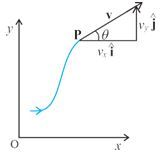
fig.4.14.The components \(v\)x and \(v\)y of velocity v and the angle \(\theta\) it makes with x-axis.
Note that \(v\)= \(v\) cos \(\theta\), \(v\)= \(v\)sin \(\theta\).
The acceleration (instantaneous acceleration) is the limiting value of the average acceleration as the time interval approaches zer:
\(% MathType!MTEF!2!1!+- % feaagKart1ev2aaatCvAUfeBSjuyZL2yd9gzLbvyNv2CaerbuLwBLn % hiov2DGi1BTfMBaeXatLxBI9gBaerbd9wDYLwzYbItLDharqqtubsr % 4rNCHbGeaGqiVu0Je9sqqrpepC0xbbL8F4rqqrFfpeea0xe9Lq-Jc9 % vqaqpepm0xbba9pwe9Q8fs0-yqaqpepae9pg0FirpepeKkFr0xfr-x % fr-xb9adbaqaaeGaciGaaiaabeqaamaabaabaaGceaqabeaacaWGHb % Gaeyypa0ZaaCbiaeaacqGHuoarcaWG0bGaeyOKH4QaaGimaaWcbeqa % aiGacYgacaGGPbGaaiyBaaaakmaalaaabaGaeyiLdqKaamODaaqaai % abgs5aejaadshaaaaabaGaci4uaiaacMgacaGGUbGaam4yaiaadwga % cqGHuoarcaWG2bGaeyypa0JaeyiLdqKaamODamaaBaaaleaacaWG4b % aabeaakiqadMgagaqcaiabgUcaRiabgs5aejaadAhadaWgaaWcbaGa % amyEaaqabaGcceWGQbGbaKaacaGGSaGaam4DaiaadwgacaaMc8UaaG % PaVlaadIgacaWGHbGaamODaiaadwgaaeaacaWGHbGaeyypa0JabmyA % ayaajaWaaCbiaeaacqGHuoarcaWG0bGaeyOKH4QaaGimaaWcbeqaai % GacYgacaGGPbGaaiyBaaaakmaalaaabaGaeyiLdqKaamODamaaBaaa % leaacaWG4baabeaaaOqaaiabgs5aejaadshaaaGaey4kaSIabmOAay % aajaWaaCbiaeaacqGHuoarcaWG0bGaeyOKH4QaaGimamaalaaabaGa % eyiLdqKaamODamaaBaaaleaacaWG5baabeaaaOqaaiabgs5aejaads % haaaaaleqabaGaciiBaiaacMgacaGGTbaaaaGcbaGaamyyaiabg2da % 9iaadggadaWgaaWcbaGaamiEaaqabaGcceWGPbGbaKaacqGHRaWkca % WGHbWaaSbaaSqaaiaadMhaaeqaaOGabmOAayaajaaabaGaam4Daiaa % dIgacaWGLbGaamOCaiaadwgacaGGSaGaamyyamaaBaaaleaacaWG4b % aabeaakiabg2da9maalaaabaGaamizaiaadAhadaWgaaWcbaGaamiE % aaqabaaakeaacaWGKbGaamiDaaaacaGGSaGaamyyamaaBaaaleaaca % WG5baabeaakiabg2da9maalaaabaGaamizaiaadAhadaWgaaWcbaGa % amyEaaqabaaakeaacaWGKbGaamiDaaaaaaaa!A0D6! \begin{array}{l} a = \mathop {\Delta t \to 0}\limits^{\lim } \frac{{\Delta v}}{{\Delta t}}\\ {\mathop{\rm Sin}\nolimits} ce\Delta v = \Delta {v_x}\hat i + \Delta {v_y}\hat j,we\,\,have\\ a = \hat i\mathop {\Delta t \to 0}\limits^{\lim } \frac{{\Delta {v_x}}}{{\Delta t}} + \hat j\mathop {\Delta t \to 0\frac{{\Delta {v_y}}}{{\Delta t}}}\limits^{\lim } \\ a = {a_x}\hat i + {a_y}\hat j\\ where,{a_x} = \frac{{d{v_x}}}{{dt}},{a_y} = \frac{{d{v_y}}}{{dt}} \end{array}\)
As in the case of velocity, we can understand graphically the limiting process used in defining acceleration on a graph showing the path of the object’s motion. This is shown in Figs. 4.15(a) to (d). P represents the position of the object at time t and P1, P2,P3 positions after time \(\Delta\)t 1, \(\Delta\)t2 ,\(\Delta\)t3,respectively (\(\Delta\)t1> \(\Delta\)t2>\(\Delta\)t3). The velocity vectors at points P, P1 , P2, P3 are also shown in Figs. 4.15. (a),(b) and (c). In each case of \(\Delta\)t, \(\Delta\)v is obtained using the triangle law of vector addition. By definition, the direction of average acceleration is the same as that of \(\Delta\)v. We see that as \(\Delta\)t decreases, the direction of \(\Delta\)v changes and consequently, the direction of the acceleration changes. Finally, in the limit \(\Delta\)t\(\to\)0 [Fig. 4.15(d)],the average acceleration becomes the instantaneous acceleration and has the direction as shown.

fig.4.15. The average acceleration for three time intervals (a) \(\Delta\)t1, (b) \(\Delta\)t2, and (c) \(\Delta\)t3, (\(\Delta\)t1> \(\Delta\)t2> \(\Delta\)t3).
(d) In the limit \(\Delta\)t\(\to\)0, the average acceleration becomes the acceleration.
Note that in one dimension, the velocity and the acceleration of an object are always along the same straight line (either in the same direction or in the opposite direction). However, for motion in two or three,dimensions, velocity and acceleration vectors may have any angle between 0° and 180° between them.
EXAMPLE 4
The position of a particle is given by \(% MathType!MTEF!2!1!+- % feaagKart1ev2aaatCvAUfeBSjuyZL2yd9gzLbvyNv2CaerbuLwBLn % hiov2DGi1BTfMBaeXatLxBI9gBaerbd9wDYLwzYbItLDharqqtubsr % 4rNCHbGeaGqiVu0Je9sqqrpepC0xbbL8F4rqqrFfpeea0xe9Lq-Jc9 % vqaqpepm0xbba9pwe9Q8fs0-yqaqpepae9pg0FirpepeKkFr0xfr-x % fr-xb9adbaqaaeGaciGaaiaabeqaamaabaabaaGcbaGaamOCaiabg2 % da9iaaiodacaGGUaGaaGimaiaadshaceWGPbGbaKaacqGHRaWkcaaI % YaGaaiOlaiaaicdacaWG0bWaaWbaaSqabeaacaaIYaaaaOGabmOAay % aajaGaey4kaSIaaGynaiaac6cacaaIWaGabm4Aayaajaaaaa!4615! r = 3.0t\hat i + 2.0{t^2}\hat j + 5.0\hat k\) where t is in seconds and the coefficients have the proper units for r to be in metres.(a) Find v(t) and a(t) of the particle. (b) Find the magnitude and direction of v(t) at t = 1.0 s.
\(% MathType!MTEF!2!1!+- % feaagKart1ev2aaatCvAUfeBSjuyZL2yd9gzLbvyNv2CaerbuLwBLn % hiov2DGi1BTfMBaeXatLxBI9gBaerbd9wDYLwzYbItLDharqqtubsr % 4rNCHbGeaGqiVu0Je9sqqrpepC0xbbL8F4rqqrFfpeea0xe9Lq-Jc9 % vqaqpepm0xbba9pwe9Q8fs0-yqaqpepae9pg0FirpepeKkFr0xfr-x % fr-xb9adbaqaaeGaciGaaiaabeqaamaabaabaaGceaqabeaacaWG2b % WaaeWaaeaacaWG0baacaGLOaGaayzkaaGaeyypa0ZaaSaaaeaacaWG % KbGaamOCaaqaaiaadsgacaWG0baaaiabg2da9maalaaabaGaamizaa % qaaiaadsgacaWG0baaamaabmaabaGaaG4maiaac6cacaaIWaGaamiD % aiqadMgagaqcaiabgUcaRiaaikdacaGGUaGaaGimaiaadshadaahaa % WcbeqaaiaaikdaaaGcceWGQbGbaKaacqGHRaWkcaaI1aGaaiOlaiaa % icdaceWGRbGbaKaaaiaawIcacaGLPaaaaeaacqGH9aqpcaaIZaGaai % OlaiaaicdaceWGPbGbaKaacqGHRaWkcaaI0aGaaiOlaiaaicdacaWG % 0bGabmOAayaajaaabaGaamyyamaabmaabaGaamiDaaGaayjkaiaawM % caaiabg2da9maalaaabaGaamizaiaadAhaaeaacaWGKbGaamiDaaaa % cqGH9aqpcqGHRaWkcaaI0aGaaiOlaiaaicdaceWGQbGbaKaaaeaaca % WGHbGaeyypa0JaaGinaiaac6cacaaIWaGaamyBaiaadohadaahaaWc % beqaaiabgkHiTiaaigdaaaaaaaa!703B! \begin{array}{l} v\left( t \right) = \frac{{dr}}{{dt}} = \frac{d}{{dt}}\left( {3.0t\hat i + 2.0{t^2}\hat j + 5.0\hat k} \right)\\ = 3.0\hat i + 4.0t\hat j\\ a\left( t \right) = \frac{{dv}}{{dt}} = + 4.0\hat j\\ a = 4.0m{s^{ - 1}} \end{array}\)
along y-direction
At t=1.0s,\(% MathType!MTEF!2!1!+- % feaagKart1ev2aaatCvAUfeBSjuyZL2yd9gzLbvyNv2CaerbuLwBLn % hiov2DGi1BTfMBaeXatLxBI9gBaerbd9wDYLwzYbItLDharqqtubsr % 4rNCHbGeaGqiVu0Je9sqqrpepC0xbbL8F4rqqrFfpeea0xe9Lq-Jc9 % vqaqpepm0xbba9pwe9Q8fs0-yqaqpepae9pg0FirpepeKkFr0xfr-x % fr-xb9adbaqaaeGaciGaaiaabeqaamaabaabaaGcbaGaamODaiabg2 % da9iaaiodacaGGUaGaaGimaiqadMgagaqcaiabgUcaRiaaisdacaGG % UaGaaGimaiqadQgagaqcaaaa!3F29! v = 3.0\hat i + 4.0\hat j\)
It’s magnitude is \(% MathType!MTEF!2!1!+- % feaagKart1ev2aaatCvAUfeBSjuyZL2yd9gzLbvyNv2CaerbuLwBLn % hiov2DGi1BTfMBaeXatLxBI9gBaerbd9wDYLwzYbItLDharqqtubsr % 4rNCHbGeaGqiVu0Je9sqqrpepC0xbbL8F4rqqrFfpeea0xe9Lq-Jc9 % vqaqpepm0xbba9pwe9Q8fs0-yqaqpepae9pg0FirpepeKkFr0xfr-x % fr-xb9adbaqaaeGaciGaaiaabeqaamaabaabaaGcbaGaamODaiabg2 % da9maakaaabaGaaG4mamaaCaaaleqabaGaaGOmaaaakiabgUcaRiaa % isdadaahaaWcbeqaaiaaikdaaaaabeaakiabg2da9iaaiwdacaGGUa % GaamyBaiaadohadaahaaWcbeqaaiabgkHiTiaaigdaaaaaaa!4280! v = \sqrt {{3^2} + {4^2}} = 5.m{s^{ - 1}}\) and direction is \(% MathType!MTEF!2!1!+- % feaagKart1ev2aaatCvAUfeBSjuyZL2yd9gzLbvyNv2CaerbuLwBLn % hiov2DGi1BTfMBaeXatLxBI9gBaerbd9wDYLwzYbItLDharqqtubsr % 4rNCHbGeaGqiVu0Je9sqqrpepC0xbbL8F4rqqrFfpeea0xe9Lq-Jc9 % vqaqpepm0xbba9pwe9Q8fs0-yqaqpepae9pg0FirpepeKkFr0xfr-x % fr-xb9adbaqaaeGaciGaaiaabeqaamaabaabaaGcbaGaeqiUdeNaey % ypa0JaciiDaiaacggacaGGUbWaaWbaaSqabeaacqGHsislcaaIXaaa % aOWaaeWaaeaadaWcaaqaaiaadAhadaWgaaWcbaGaamyEaaqabaaake % aacaWG2bWaaSbaaSqaaiaadIhaaeqaaaaaaOGaayjkaiaawMcaaiab % g2da9iGacshacaGGHbGaaiOBamaaCaaaleqabaGaeyOeI0IaaGymaa % aakmaabmaabaWaaSaaaeaacaaI0aaabaGaaG4maaaaaiaawIcacaGL % PaaacqGHfjcqcaaI1aGaaG4mamaaCaaaleqabaGaaGimaaaaaaa!4FB8! \theta = {\tan ^{ - 1}}\left( {\frac{{{v_y}}}{{{v_x}}}} \right) = {\tan ^{ - 1}}\left( {\frac{4}{3}} \right) \cong {53^0}\) with x-axis
-
Motion in a Plane with Constant Acceleration
Motion in a Plane with Constant Acceleration
Suppose that an object is moving in x-y plane and its acceleration a is constant. Over an interval of time, the average acceleration will equal this constant value. Now, let the velocity of the object be v0 at time t = 0 and v at time t.
Then, by definition
\(% MathType!MTEF!2!1!+- % feaagKart1ev2aaatCvAUfeBSjuyZL2yd9gzLbvyNv2CaerbuLwBLn % hiov2DGi1BTfMBaeXatLxBI9gBaerbd9wDYLwzYbItLDharqqtubsr % 4rNCHbGeaGqiVu0Je9sqqrpepC0xbbL8F4rqqrFfpeea0xe9Lq-Jc9 % vqaqpepm0xbba9pwe9Q8fs0-yqaqpepae9pg0FirpepeKkFr0xfr-x % fr-xb9adbaqaaeGaciGaaiaabeqaamaabaabaaGceaqabeaacaWGHb % Gaeyypa0ZaaSaaaeaacaWG2bGaeyOeI0IaamODamaaBaaaleaacaaI % WaaabeaaaOqaaiaadshacqGHsislcaaIWaaaaiabg2da9maalaaaba % GaamODaiabgkHiTiaadAhadaWgaaWcbaGaaGimaaqabaaakeaacaWG % 0baaaaqaaiaad+eacaWGYbGaaiilaiaadAhacqGH9aqpcaWG2bWaaS % baaSqaaiaaicdaaeqaaOGaey4kaSIaamyyaiaadshaaaaa!4D76! \begin{array}{l} a = \frac{{v - {v_0}}}{{t - 0}} = \frac{{v - {v_0}}}{t}\\ Or,v = {v_0} + at \end{array}\)
In terms of components :
\(v\)x=\(v\)ox + axt
\(v\)y=\(v\)oy + ayt
Let us now find how the position r changes with time. We follow the method used in the one- dimensional case. Let ro and r be the position vectors of the particle at time 0 and t and let the velocities at these instants be vo and v. Then, over this time interval t, the average velocity is (\(v\)o + \(v\))/2. The displacement is the average velocity multiplied by the time interval :
\(% MathType!MTEF!2!1!+- % feaagKart1ev2aaatCvAUfeBSjuyZL2yd9gzLbvyNv2CaerbuLwBLn % hiov2DGi1BTfMBaeXatLxBI9gBaerbd9wDYLwzYbItLDharqqtubsr % 4rNCHbGeaGqiVu0Je9sqqrpepC0xbbL8F4rqqrFfpeea0xe9Lq-Jc9 % vqaqpepm0xbba9pwe9Q8fs0-yqaqpepae9pg0FirpepeKkFr0xfr-x % fr-xb9adbaqaaeGaciGaaiaabeqaamaabaabaaGceaqabeaaqaaaaa % aaaaWdbiaadkhacqGHsislcaWGYbWaaSbaaSqaaiaaicdaaeqaaOGa % eyypa0ZaaeWaaeaadaWcaaqaaiaadAhacqGHRaWkcaWG2bWaaSbaaS % qaaiaaicdaaeqaaaGcbaGaaGOmaaaaaiaawIcacaGLPaaacaWG0bGa % eyypa0ZaaeWaaeaadaWcaaqaamaabmaabaGaamODamaaBaaaleaaca % aIWaaabeaakiabgUcaRiaadggacaWG0baacaGLOaGaayzkaaGaey4k % aSIaamODamaaBaaaleaacaaIWaaabeaaaOqaaiaaikdaaaaacaGLOa % GaayzkaaGaamiDaaqaaiabg2da9iaadAhadaWgaaWcbaGaaGimaaqa % baGccaWG0bGaey4kaSYaaSaaaeaacaaIXaaabaGaaGOmaaaacaWGHb % GaamiDamaaCaaaleqabaGaaGOmaaaaaOqaaiaad+eacaWGYbGaaiil % aiaadkhacqGH9aqpcaWGYbWaaSbaaSqaaiaaicdaaeqaaOGaey4kaS % IaamODamaaBaaaleaacaaIWaaabeaakiaadshacqGHRaWkdaWcaaqa % aiaaigdaaeaacaaIYaaaaiaadggacaWG0bWaaWbaaSqabeaacaaIYa % aaaaaaaa!67D6! \begin{array}{l} r - {r_0} = \left( {\frac{{v + {v_0}}}{2}} \right)t = \left( {\frac{{\left( {{v_0} + at} \right) + {v_0}}}{2}} \right)t\\ = {v_0}t + \frac{1}{2}a{t^2}\\ Or,r = {r_0} + {v_0}t + \frac{1}{2}a{t^2} \end{array}\)
It can be easily verified that the derivative of Eq. (4.34a), i.e.\(% MathType!MTEF!2!1!+- % feaagKart1ev2aaatCvAUfeBSjuyZL2yd9gzLbvyNv2CaerbuLwBLn % hiov2DGi1BTfMBaeXatLxBI9gBaerbd9wDYLwzYbItLDharqqtubsr % 4rNCHbGeaGqiVu0Je9sqqrpepC0xbbL8F4rqqrFfpeea0xe9Lq-Jc9 % vqaqpepm0xbba9pwe9Q8fs0-yqaqpepae9pg0FirpepeKkFr0xfr-x % fr-xb9adbaqaaeGaciGaaiaabeqaamaabaabaaGcbaaeaaaaaaaaa8 % qadaWcaaqaaiaadsgacaWGYbaabaGaamizaiaadshaaaaaaa!39E8! \frac{{dr}}{{dt}}\) gives Eq.(4.33a) and it also satisfies the condition that at t=0, r = ro.
Equation (4.34a) can be written in component form as
\(% MathType!MTEF!2!1!+- % feaagKart1ev2aaatCvAUfeBSjuyZL2yd9gzLbvyNv2CaerbuLwBLn % hiov2DGi1BTfMBaeXatLxBI9gBaerbd9wDYLwzYbItLDharqqtubsr % 4rNCHbGeaGqiVu0Je9sqqrpepC0xbbL8F4rqqrFfpeea0xe9Lq-Jc9 % vqaqpepm0xbba9pwe9Q8fs0-yqaqpepae9pg0FirpepeKkFr0xfr-x % fr-xb9adbaqaaeGaciGaaiaabeqaamaabaabaaGceaqabeaaqaaaaa % aaaaWdbiaadIhacqGH9aqpcaWG4bWaaSbaaSqaaiaaicdaaeqaaOGa % ey4kaSIaamODamaaBaaaleaacaWGHbGaamiEaaqabaGccaWG0bGaey % 4kaSYaaSaaaeaacaaIXaaabaGaaGOmaaaacaWGHbWaaSbaaSqaaiaa % dIhaaeqaaOGaamiDamaaCaaaleqabaGaaGOmaaaaaOqaaiaadMhacq % GH9aqpcaWG5bWaaSbaaSqaaiaaicdaaeqaaOGaey4kaSIaamODamaa % BaaaleaacaWGHbGaamyEaaqabaGccaWG0bGaey4kaSYaaSaaaeaaca % aIXaaabaGaaGOmaaaacaWGHbWaaSbaaSqaaiaadMhaaeqaaOGaamiD % amaaCaaaleqabaGaaGOmaaaaaaaa!54B1! \begin{array}{l} x = {x_0} + {v_{ax}}t + \frac{1}{2}{a_x}{t^2}\\ y = {y_0} + {v_{ay}}t + \frac{1}{2}{a_y}{t^2} \end{array}\)
One immediate interpretation of Eq.(4.34b) is that the motions in x- and y-directions can be treated independently of each other. That is, motion in a plane (two-dimensions) can be treated as two separate simultaneous one-dimensional motions with constant acceleration along two perpendicular directions. This is an important result and is useful in analysing motion of objects in two dimensions. A similar result holds for three dimensions.The choice of perpendicular directions is convenient in many physical situations, as we shall see in section 4.10 for projectile motion.
EXAMPLE 5
A particle starts from origin at t = 0 with a velocity 5.0 î m/s and moves in x-y plane under action of a force which produces a constant acceleration of (3.0\(\hat i\)+2.0\(\hat j\) )m/s 2. (a)What is the y-coordinate of the particle at the instant its x-coordinate is 84 m ? (b) What is the speed of the particle at this time ?
ANSWER
From Eq. (4.34a) for r0 = 0,the position of the particle is given by
\(% MathType!MTEF!2!1!+- % feaagKart1ev2aaatCvAUfeBSjuyZL2yd9gzLbvyNv2CaerbuLwBLn % hiov2DGi1BTfMBaeXatLxBI9gBaerbd9wDYLwzYbItLDharqqtubsr % 4rNCHbGeaGqiVu0Je9sqqrpepC0xbbL8F4rqqrFfpeea0xe9Lq-Jc9 % vqaqpepm0xbba9pwe9Q8fs0-yqaqpepae9pg0FirpepeKkFr0xfr-x % fr-xb9adbaqaaeGaciGaaiaabeqaamaabaabaaGceaqabeaaqaaaaa % aaaaWdbiaadkhadaqadaqaaiaadshaaiaawIcacaGLPaaacqGH9aqp % caWG2bWaaSbaaSqaaiaaicdaaeqaaOGaamiDaiabgUcaRmaalaaaba % GaaGymaaqaaiaaikdaaaGaamyyaiaadshadaahaaWcbeqaaiaaikda % aaaakeaacqGH9aqpcaaI1aGaaiOlaiaaicdaceWGPbGbaKaacaWG0b % Gaey4kaSYaaeWaaeaacaaIXaGaai4laiaaikdaaiaawIcacaGLPaaa % daqadaqaaiaaiodacaGGUaGaaGimaiqadMgagaqcaiabgUcaRiaaik % dacaGGUaGaaGimaiqadQgagaqcaaGaayjkaiaawMcaaiaadshadaah % aaWcbeqaaiaaikdaaaaakeaacqGH9aqpdaqadaqaaiaaiwdacaGGUa % GaaGimaiaadshacqGHRaWkcaaIXaGaaiOlaiaaiwdacaWG0bWaaWba % aSqabeaacaaIYaaaaaGccaGLOaGaayzkaaGabmyAayaajaGaey4kaS % IaaGymaiaac6cacaaIWaGaamiDamaaCaaaleqabaGaaGOmaaaakiqa % dQgagaqcaaqaaiaadsfacaWGObGaamyzaiaadkhacaWGLbGaamOzai % aad+gacaWGYbGaamyzaiaacYcacaWG4bWaaeWaaeaacaWG0baacaGL % OaGaayzkaaGaeyypa0JaaGynaiaac6cacaaIWaGaamiDaiabgUcaRi % aaigdacaGGUaGaaGynaiaadshadaahaaWcbeqaaiaaikdaaaaakeaa % caWG5bWaaeWaaeaacaWG0baacaGLOaGaayzkaaGaeyypa0Jaey4kaS % IaaGymaiaac6cacaaIWaGaamiDamaaCaaaleqabaGaaGOmaaaaaaaa % !87D4! \begin{array}{l} r\left( t \right) = {v_0}t + \frac{1}{2}a{t^2}\\ = 5.0\hat it + \left( {1/2} \right)\left( {3.0\hat i + 2.0\hat j} \right){t^2}\\ = \left( {5.0t + 1.5{t^2}} \right)\hat i + 1.0{t^2}\hat j\\ Therefore,x\left( t \right) = 5.0t + 1.5{t^2}\\ y\left( t \right) = + 1.0{t^2} \end{array}\)
Givenx (t) = 84 m, t = ?
5.0 t + 1.5 t2 = 84 \(\Rightarrow\)t = 6 s
At t = 6 s, y = 1.0 (6)2 = 36.0 m
Now, the velocity \(% MathType!MTEF!2!1!+- % feaagKart1ev2aaatCvAUfeBSjuyZL2yd9gzLbvyNv2CaerbuLwBLn % hiov2DGi1BTfMBaeXatLxBI9gBaerbd9wDYLwzYbItLDharqqtubsr % 4rNCHbGeaGqiVu0Je9sqqrpepC0xbbL8F4rqqrFfpeea0xe9Lq-Jc9 % vqaqpepm0xbba9pwe9Q8fs0-yqaqpepae9pg0FirpepeKkFr0xfr-x % fr-xb9adbaqaaeGaciGaaiaabeqaamaabaabaaGcbaGaamODaiabg2 % da9maalaaabaGaamizaiaadkhaaeaacaWGKbGaamiDaaaacqGH9aqp % daqadaqaaiaaiwdacaGGUaGaaGimaiabgUcaRiaaiodacaGGUaGaaG % imaiaadshaaiaawIcacaGLPaaaceWGPbGbaKaacqGHRaWkcaaIYaGa % aiOlaiaaicdacaWG0bGabmOAayaajaaaaa!4A87! v = \frac{{dr}}{{dt}} = \left( {5.0 + 3.0t} \right)\hat i + 2.0t\hat j\)
At t=6s,v=23.0\(\hat i\)+12.0\(\hat j\)
\(% MathType!MTEF!2!1!+- % feaagKart1ev2aaatCvAUfeBSjuyZL2yd9gzLbvyNv2CaerbuLwBLn % hiov2DGi1BTfMBaeXatLxBI9gBaerbd9wDYLwzYbItLDharqqtubsr % 4rNCHbGeaGqiVu0Je9sqqrpepC0xbbL8F4rqqrFfpeea0xe9Lq-Jc9 % vqaqpepm0xbba9pwe9Q8fs0-yqaqpepae9pg0FirpepeKkFr0xfr-x % fr-xb9adbaqaaeGaciGaaiaabeqaamaabaabaaGcbaGaam4Caiaadc % hacaWGLbGaamyzaiaadsgacqGH9aqpdaabdaqaaiaadAhaaiaawEa7 % caGLiWoacqGH9aqpdaGcaaqaaiaaikdacaaIZaWaaWbaaSqabeaaca % aIYaaaaOGaey4kaSIaaGymaiaaikdadaahaaWcbeqaaiaaikdaaaaa % beaakiabgwKiajaaikdacaaI2aGaamyBaiaadohadaahaaWcbeqaai % abgkHiTiaaigdaaaaaaa!4CFF! speed = \left| v \right| = \sqrt {{{23}^2} + {{12}^2}} \cong 26m{s^{ - 1}}\)
-
Relative Velocity in Two Dimensions
Relative Velocity in Two Dimensions
The concept of relative velocity, introduced in section 3.7 for motion along a straight line, can be easily extended to include motion in a plane
or in three dimensions. Suppose that two objects A and B are moving with velocities v A and v B (each with respect to some common frame of reference, say ground.).
Then, velocity of object A relative to that of B is :vAB=vA-vB
and similarly, the velocity of object B relative to that of A is :vBA=vB-vA
Therefore,vAB=-vBA and \(% MathType!MTEF!2!1!+- % feaagKart1ev2aaatCvAUfeBSjuyZL2yd9gzLbvyNv2CaerbuLwBLn % hiov2DGi1BTfMBaeXatLxBI9gBaerbd9wDYLwzYbItLDharqqtubsr % 4rNCHbGeaGqiVu0Je9sqqrpepC0xbbL8F4rqqrFfpeea0xe9Lq-Jc9 % vqaqpepm0xbba9pwe9Q8fs0-yqaqpepae9pg0FirpepeKkFr0xfr-x % fr-xb9adbaqaaeGaciGaaiaabeqaamaabaabaaGcbaWaaqWaaeaaca % WG2bWaaSbaaSqaaiaadgeacaWGcbaabeaaaOGaay5bSlaawIa7aiab % g2da9maaemaabaGaamODamaaBaaaleaacaWGcbGaamyqaaqabaaaki % aawEa7caGLiWoaaaa!42BC! \left| {{v_{AB}}} \right| = \left| {{v_{BA}}} \right|\)
EXAMPLE 6
Rain is falling vertically with a speed of 35 m s–1. A woman rides a bicycle with a speed of 12 m s–1 in east to west direction. What is the direction in which she should hold her umbrella ?
ANSWER
In Fig. 4.16 vr represents the velocity of rain and vb, the velocity of the bicycle, the woman is riding. Both these velocities are with
respect to the ground. Since the woman is riding a bicycle, the velocity of rain as experienced by her is the velocity of rain relative to the velocity of the bicycle she is riding. That is vrb = vr – vb.
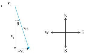
fig.4.16.
This relative velocity vector as shown in Fig. 4.16 makes an angle \(\theta\) with the vertical. It is given by
\(% MathType!MTEF!2!1!+- % feaagKart1ev2aaatCvAUfeBSjuyZL2yd9gzLbvyNv2CaerbuLwBLn % hiov2DGi1BTfMBaeXatLxBI9gBaerbd9wDYLwzYbItLDharqqtubsr % 4rNCHbGeaGqiVu0Je9sqqrpepC0xbbL8F4rqqrFfpeea0xe9Lq-Jc9 % vqaqpepm0xbba9pwe9Q8fs0-yqaqpepae9pg0FirpepeKkFr0xfr-x % fr-xb9adbaqaaeGaciGaaiaabeqaamaabaabaaGceaqabeaaciGG0b % Gaaiyyaiaac6gacqaH4oqCcqGH9aqpdaWcaaqaaiaadAhadaWgaaWc % baGaamOyaaqabaaakeaacaWG2bWaaSbaaSqaaiaadkhaaeqaaaaaki % abg2da9maalaaabaGaaGymaiaaikdaaeaacaaIZaGaaGynaaaacqGH % 9aqpcaaIWaGaaiOlaiaaiodacaaI0aGaaG4maaqaaiaad+eacaWGYb % GaaiilaiabeI7aXjabgwKiajaaigdacaaI5aWaaWbaaSqabeaacaaI % Waaaaaaaaa!5056! \begin{array}{l} \tan \theta = \frac{{{v_b}}}{{{v_r}}} = \frac{{12}}{{35}} = 0.343\\ Or,\theta \cong {19^0} \end{array}\)
Therefore, the woman should hold her umbrella at an angle of about 19° with the vertical towards the west.
Note carefully the difference between this Example and the Example 4.1. In Example 4.1, the boy experiences the resultant (vectorsum) of two velocities while in this example,the woman experiences the velocity of rain relative to the bicycle (the vector difference of the two velocities).