Explanation of Magnetic Field of a Circular Current Loop

Explanation of Magnetic Field of a Circular Current Loop

In this section, we shall evaluate the magnetic field due to a circular coil along its axis. The evaluation entails summing up the effect of infinitesimal current elements (I dl) mentioned in the previous section.

We assume that the current I is steady and that the evaluation is carried out in free space (i.e., vacuum).

Figure 4.11 depicts a circular loop carrying a steady current I. The loop is placed in the y-z plane with its centre at the origin O and has a radius R. The x-axis is the axis of the loop. We wish to calculate the magnetic field at the point P on this axis. Let x be the distance of P from the centre O of the loop.

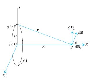
                 Figure 4.11

Consider a conducting element dl of the loop. This is shown in Fig. 4.11. The magnitude dB of the magnetic field due to dl is given by the Biot-Savart law [Eq. 4.11(a)], 

\(% MathType!MTEF!2!1!+- % feaagKart1ev2aaatCvAUfeBSjuyZL2yd9gzLbvyNv2CaerbuLwBLn % hiov2DGi1BTfMBaeXatLxBI9gBaerbd9wDYLwzYbItLDharqqtubsr % 4rNCHbGeaGqiVu0Je9sqqrpepC0xbbL8F4rqqrFfpeea0xe9Lq-Jc9 % vqaqpepm0xbba9pwe9Q8fs0-yqaqpepae9pg0FirpepeKkFr0xfr-x % fr-xb9adbaqaaeGaciGaaiaabeqaamaabaabaaGcbaaeaaaaaaaaa8 % qacaWGKbGaamOqaiabg2da9maalaaabaGaeqiVd02aaSbaaSqaaiaa % icdaaeqaaaGcbaGaaGinaiabec8aWbaadaWcaaqaaiaadMeadaabda % qaaiaadsgacaWGSbGaey41aqRaamOCaaGaay5bSlaawIa7aaqaaiaa % dkhadaahaaWcbeqaaiaaiodaaaaaaaaa!48C6! dB = \frac{{{\mu _0}}}{{4\pi }}\frac{{I\left| {dl \times r} \right|}}{{{r^3}}}\)      (4.12)

Now r ² = x ² + R ² . Further, any element of the loop will be perpendicular to the displacement vector from the element to the axial point. For example, the element dl in Fig. 4.11 is in the y-z plane, whereas, the displacement vector r from dl to the axial point P is in the x-y plane. Hence |dl × r|=r dl. Thus,

\(% MathType!MTEF!2!1!+- % feaagKart1ev2aaatCvAUfeBSjuyZL2yd9gzLbvyNv2CaerbuLwBLn % hiov2DGi1BTfMBaeXatLxBI9gBaerbd9wDYLwzYbItLDharqqtubsr % 4rNCHbGeaGqiVu0Je9sqqrpepC0xbbL8F4rqqrFfpeea0xe9Lq-Jc9 % vqaqpepm0xbba9pwe9Q8fs0-yqaqpepae9pg0FirpepeKkFr0xfr-x % fr-xb9adbaqaaeGaciGaaiaabeqaamaabaabaaGcbaaeaaaaaaaaa8 % qacaWGKbGaamOqaiabg2da9maalaaabaGaeqiVd02aaSbaaSqaaiaa % icdaaeqaaaGcbaGaaGinaiabec8aWbaadaWcaaqaaiaadMeacaWGKb % GaamiBaaqaamaabmaabaGaamiEamaaCaaaleqabaGaaGOmaaaakiab % gUcaRiaadkfadaahaaWcbeqaaiaaikdaaaaakiaawIcacaGLPaaaaa % aaaa!46DA! dB = \frac{{{\mu _0}}}{{4\pi }}\frac{{Idl}}{{\left( {{x^2} + {R^2}} \right)}}\)       (4.13)

The direction of dB is shown in Fig. 4.11. It is perpendicular to the plane formed by dl and r. It has an x-component dB_x and a component perpendicular to x-axis, dB\(% MathType!MTEF!2!1!+- % feaagKart1ev2aaatCvAUfeBSjuyZL2yd9gzLbvyNv2CaerbuLwBLn % hiov2DGi1BTfMBaeXatLxBI9gBaerbd9wDYLwzYbItLDharqqtubsr % 4rNCHbGeaGqiVu0Je9sqqrpepC0xbbL8F4rqqrFfpeea0xe9Lq-Jc9 % vqaqpepm0xbba9pwe9Q8fs0-yqaqpepae9pg0FirpepeKkFr0xfr-x % fr-xb9adbaqaaeGaciGaaiaabeqaamaabaabaaGcbaaeaaaaaaaaa8 % qadaWgaaWcbaGaeyyPI4fabeaaaaa!37F3! _ \bot \) When the components perpendicular to the x-axis are summed over, they cancel out and we obtain a null result. For example, the dB\(% MathType!MTEF!2!1!+- % feaagKart1ev2aaatCvAUfeBSjuyZL2yd9gzLbvyNv2CaerbuLwBLn % hiov2DGi1BTfMBaeXatLxBI9gBaerbd9wDYLwzYbItLDharqqtubsr % 4rNCHbGeaGqiVu0Je9sqqrpepC0xbbL8F4rqqrFfpeea0xe9Lq-Jc9 % vqaqpepm0xbba9pwe9Q8fs0-yqaqpepae9pg0FirpepeKkFr0xfr-x % fr-xb9adbaqaaeGaciGaaiaabeqaamaabaabaaGcbaaeaaaaaaaaa8 % qadaWgaaWcbaGaeyyPI4fabeaaaaa!37F3! _ \bot \) component due to dl is cancelled by the contribution due to the  diametrically  opposite  d l element,  shown in Fig. 4.11. Thus, only the x-component survives. The net contribution along x-direction can be obtained by integrating dB_x = dB cos\(\theta\) over the loop. For Fig. 4.11,

\(% MathType!MTEF!2!1!+- % feaagKart1ev2aaatCvAUfeBSjuyZL2yd9gzLbvyNv2CaerbuLwBLn % hiov2DGi1BTfMBaeXatLxBI9gBaerbd9wDYLwzYbItLDharqqtubsr % 4rNCHbGeaGqiVu0Je9sqqrpepC0xbbL8F4rqqrFfpeea0xe9Lq-Jc9 % vqaqpepm0xbba9pwe9Q8fs0-yqaqpepae9pg0FirpepeKkFr0xfr-x % fr-xb9adbaqaaeGaciGaaiaabeqaamaabaabaaGcbaaeaaaaaaaaa8 % qaciGGJbGaai4BaiaacohacqaH4oqCcqGH9aqpdaWcaaqaaiaadkfa % aeaadaqadaqaaiaadIhadaahaaWcbeqaaiaaikdaaaGccqGHRaWkca % WGsbWaaWbaaSqabeaacaaIYaaaaaGccaGLOaGaayzkaaWaaWbaaSqa % beaacaaIXaGaai4laiaaikdaaaaaaOGaaGPaVlaaykW7caaMc8UaaG % PaVlaaykW7caaMc8UaaGPaVlaaykW7caaMc8UaaGPaVlaaykW7caaM % c8UaaGPaVlaaykW7caaMc8UaaGPaVlaaykW7caaMc8UaaGPaVlaayk % W7caaMc8UaaGPaVlaaykW7caaMc8UaaGPaVpaabmaabaGaaGinaiaa % c6cacaaIXaGaaGinaaGaayjkaiaawMcaaaaa!7017! \cos \theta = \frac{R}{{{{\left( {{x^2} + {R^2}} \right)}^{1/2}}}}\,\,\,\,\,\,\,\,\,\,\,\,\,\,\,\,\,\,\,\,\,\,\,\,\,\left( {4.14} \right)\)

From Eqs. (4.13) and (4.14),

\(% MathType!MTEF!2!1!+- % feaagKart1ev2aaatCvAUfeBSjuyZL2yd9gzLbvyNv2CaerbuLwBLn % hiov2DGi1BTfMBaeXatLxBI9gBaerbd9wDYLwzYbItLDharqqtubsr % 4rNCHbGeaGqiVu0Je9sqqrpepC0xbbL8F4rqqrFfpeea0xe9Lq-Jc9 % vqaqpepm0xbba9pwe9Q8fs0-yqaqpepae9pg0FirpepeKkFr0xfr-x % fr-xb9adbaqaaeGaciGaaiaabeqaamaabaabaaGcbaaeaaaaaaaaa8 % qacaWGKbGaamOqamaaBaaaleaacaWG4baabeaakiabg2da9maalaaa % baGaeqiVd02aaSbaaSqaaiaaicdaaeqaaOGaamysaiaadsgacaWGSb % aabaGaaGinaiabec8aWbaadaWcaaqaaiaadkfaaeaadaqadaqaaiaa % dIhadaahaaWcbeqaaiaaikdaaaGccqGHRaWkcaWGsbWaaWbaaSqabe % aacaaIYaaaaaGccaGLOaGaayzkaaWaaWbaaSqabeaacaaIZaGaai4l % aiaaikdaaaaaaaaa!4B3D! d{B_x} = \frac{{{\mu _0}Idl}}{{4\pi }}\frac{R}{{{{\left( {{x^2} + {R^2}} \right)}^{3/2}}}}\)

The summation of elements dl over the loop yields 2\(\pi\)R, the circumference of the loop. Thus, the magnetic field at P due to entire circular loop is

\(% MathType!MTEF!2!1!+- % feaagKart1ev2aaatCvAUfeBSjuyZL2yd9gzLbvyNv2CaerbuLwBLn % hiov2DGi1BTfMBaeXatLxBI9gBaerbd9wDYLwzYbItLDharqqtubsr % 4rNCHbGeaGqiVu0Je9sqqrpepC0xbbL8F4rqqrFfpeea0xe9Lq-Jc9 % vqaqpepm0xbba9pwe9Q8fs0-yqaqpepae9pg0FirpepeKkFr0xfr-x % fr-xb9adbaqaaeGaciGaaiaabeqaamaabaabaaGcbaGaamOqaiabg2 % da9iaadkeadaWgaaWcbaGaamiEaaqabaGcceWGPbGbaKaacqGH9aqp % daWcaaqaaiabeY7aTnaaBaaaleaacaaIWaaabeaakiaadMeacaWGsb % WaaWbaaSqabeaacaaIYaaaaaGcbaGaaGOmamaabmaabaGaamiEamaa % CaaaleqabaGaaGOmaaaakiabgUcaRiaadkfadaahaaWcbeqaaiaaik % daaaaakiaawIcacaGLPaaadaahaaWcbeqaaiaaiodacaGGVaGaaGOm % aaaaaaGcceWGPbGbaKaaaaa!4B51! B = {B_x}\hat i = \frac{{{\mu _0}I{R^2}}}{{2{{\left( {{x^2} + {R^2}} \right)}^{3/2}}}}\hat i\)   (4.15)

As a special case of the above result, we may obtain the field at the center of the loop. Here x = 0, and we obtain, 

\(% MathType!MTEF!2!1!+- % feaagKart1ev2aaatCvAUfeBSjuyZL2yd9gzLbvyNv2CaerbuLwBLn % hiov2DGi1BTfMBaeXatLxBI9gBaerbd9wDYLwzYbItLDharqqtubsr % 4rNCHbGeaGqiVu0Je9sqqrpepC0xbbL8F4rqqrFfpeea0xe9Lq-Jc9 % vqaqpepm0xbba9pwe9Q8fs0-yqaqpepae9pg0FirpepeKkFr0xfr-x % fr-xb9adbaqaaeGaciGaaiaabeqaamaabaabaaGcbaGaamOqamaaBa % aaleaacaaIWaaabeaakiabg2da9maalaaabaGaeqiVd02aaSbaaSqa % aiaaicdaaeqaaOGaamysaaqaaiaaikdacaWGsbaaaiqadMgagaqcaa % aa!3EC8! {B_0} = \frac{{{\mu _0}I}}{{2R}}\hat i\)     (4.16)

The magnetic field lines due to a circular wire form closed loops and are shown in Fig. 4.12. The direction of the magnetic field is given by (another) right-hand thumb rule stated below:

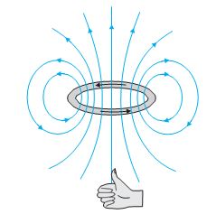
FIGURE 4.12 The magnetic field lines for a current loop. The direction of the field is given by the right-hand thumb rule described in the text. The upper side of the loop may be thought of as the north pole and the lower side as the south pole of a magnet.

Curl the palm of your right hand around the circular wire with the fingers pointing in the direction of the current. The right-hand thumb 

gives the direction of the magnetic field.

EXAMPLE 6

A straight wire carrying a current of 12 A is bent into a semi-circular arc of radius 2.0 cm as shown in Fig. 4.13(a). Consider the magnetic field B at the centre of the arc. (a) What is the magnetic field due to the straight segments? (b) In what way the contribution to B from the semicircle differs from that of a circular loop and in what way does it resemble? (c) Would your answer be different if the wire were bent into a semi-circular arc of the same radius but in the opposite way as shown in Fig. 4.13(b)?

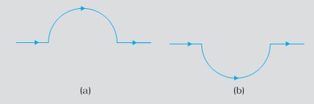
                             Fig. 4.13

Solution

a. dl and r for each element of the straight segments are parallel. Therefore, dl × r = 0. Straight segments do not contribute to

|B|.

b. For all segments of the semicircular arc, dl × r are all parallel to each other (into the plane of the paper). All such contributions add up in magnitude. Hence direction of B for a semicircular arc is given by the right-hand rule and magnitude is half that of a circular loop. Thus B is 1.9 × 10^–4 T normal to the plane of the paper going into it.

c. Same magnitude of B but opposite in direction to that in (b).

EXAMPLE 7

Consider a tightly wound 100 turn coil of radius 10 cm, carrying a current of 1 A. What is the magnitude of the magnetic field at the centre of the coil?

SOLUTION

Since the coil is tightly wound, we may take each circular element to have the same radius R = 10 cm = 0.1 m. The number of turns N = 100. The magnitude of the magnetic field is,

\(% MathType!MTEF!2!1!+- % feaagKart1ev2aaatCvAUfeBSjuyZL2yd9gzLbvyNv2CaerbuLwBLn % hiov2DGi1BTfMBaeXatLxBI9gBaerbd9wDYLwzYbItLDharqqtubsr % 4rNCHbGeaGqiVu0Je9sqqrpepC0xbbL8F4rqqrFfpeea0xe9Lq-Jc9 % vqaqpepm0xbba9pwe9Q8fs0-yqaqpepae9pg0FirpepeKkFr0xfr-x % fr-xb9adbaqaaeGaciGaaiaabeqaamaabaabaaGcbaGaamOqaiabg2 % da9maalaaabaGaeqiVd02aaSbaaSqaaiaaicdaaeqaaOGaamOtaiaa % dMeaaeaacaaIYaGaamOuaaaacqGH9aqpdaWcaaqaaiaaisdacqaHap % aCcqGHxdaTcaaIXaGaaGimamaaCaaaleqabaGaeyOeI0IaaG4naaaa % kiabgEna0kaaigdacaaIWaWaaWbaaSqabeaacaaIYaaaaOGaey41aq % RaaGymaaqaaiaaikdacqGHxdaTcaaIXaGaaGimamaaCaaaleqabaGa % eyOeI0IaaGymaaaaaaGccqGH9aqpcaaIYaGaeqiWdaNaey41aqRaaG % ymaiaaicdadaahaaWcbeqaaiabgkHiTiaaisdaaaGccqGH9aqpcaaI % 2aGaaiOlaiaaikdacaaI4aGaey41aqRaaGymaiaaicdadaahaaWcbe % qaaiabgkHiTiaaisdaaaGccaWGubaaaa!6751! B = \frac{{{\mu _0}NI}}{{2R}} = \frac{{4\pi \times {{10}^{ - 7}} \times {{10}^2} \times 1}}{{2 \times {{10}^{ - 1}}}} = 2\pi \times {10^{ - 4}} = 6.28 \times {10^{ - 4}}T\)