-
Explanation of Magnetic Flux
Explanation of Magnetic Flux
Faraday’s great insight lay in discovering a simple mathematical relation to explain the series of experiments he carried out on electromagnetic induction. However, before we state and appreciate his laws, we must get familiar with the notion of magnetic flux, \(% MathType!MTEF!2!1!+- % feaagKart1ev2aaatCvAUfeBSjuyZL2yd9gzLbvyNv2CaerbuLwBLn % hiov2DGi1BTfMBaeXatLxBI9gBaerbd9wDYLwzYbItLDharqqtubsr % 4rNCHbGeaGqiVu0Je9sqqrpepC0xbbL8F4rqqrFfpeea0xe9Lq-Jc9 % vqaqpepm0xbba9pwe9Q8fs0-yqaqpepae9pg0FirpepeKkFr0xfr-x % fr-xb9adbaqaaeGaciGaaiaabeqaamaabaabaaGcbaGaeuOPdy0aaS % baaSqaaiaadkeaaeqaaaaa!3863! {\Phi _B}\). Magnetic flux is defined in the same way as electric flux is defined in Chapter 1. Magnetic flux through a plane of area A placed in a uniform magnetic field B (Fig. 6.4) can be written as
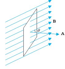
FIGURE 6.4 A plane of surface area A placed in a uniform magnetic field B.
\(% MathType!MTEF!2!1!+- % feaagKart1ev2aaatCvAUfeBSjuyZL2yd9gzLbvyNv2CaerbuLwBLn % hiov2DGi1BTfMBaeXatLxBI9gBaerbd9wDYLwzYbItLDharqqtubsr % 4rNCHbGeaGqiVu0Je9sqqrpepC0xbbL8F4rqqrFfpeea0xe9Lq-Jc9 % vqaqpepm0xbba9pwe9Q8fs0-yqaqpepae9pg0FirpepeKkFr0xfr-x % fr-xb9adbaqaaeGaciGaaiaabeqaamaabaabaaGcbaGaeuOPdy0aaS % baaSqaaiaadkeaaeqaaaaa!3863! {\Phi _B}\) = B . A = BA cos \(\theta\) (6.1)
where \(\theta\) is angle between B and A. The notion of the area as a vector has been discussed earlier in Chapter 1. Equation (6.1) can be extended to curved surfaces and nonuniform fields.
If the magnetic field has different magnitudes and directions at various parts of a surface as shown in Fig. 6.5, then the magnetic flux through the surface is given by
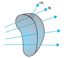
FIGURE 6.5 Magnetic field Bi at the ith area element. dA represents area vector of the ith area element.
\(% MathType!MTEF!2!1!+- % feaagKart1ev2aaatCvAUfeBSjuyZL2yd9gzLbvyNv2CaerbuLwBLn % hiov2DGi1BTfMBaeXatLxBI9gBaerbd9wDYLwzYbItLDharqqtubsr % 4rNCHbGeaGqiVu0Je9sqqrpepC0xbbL8F4rqqrFfpeea0xe9Lq-Jc9 % vqaqpepm0xbba9pwe9Q8fs0-yqaqpepae9pg0FirpepeKkFr0xfr-x % fr-xb9adbaqaaeGaciGaaiaabeqaamaabaabaaGcbaGaeuOPdy0aaS % baaSqaaiaadkeaaeqaaOGaeyypa0JaamOqamaaBaaaleaacaWGPbaa % beaakiaac6cacaWGKbGaamyqamaaBaaaleaacaWGPbaabeaakiabgU % caRiaadkeadaWgaaWcbaGaaGOmaaqabaGccaGGUaGaamizaiaadgea % daWgaaWcbaGaaGOmaaqabaGccqGHRaWkcaGGUaGaaiOlaiaac6caca % GGUaGaaiOlaiaac6cacaGGUaGaaiOlaiaac6cacaGGUaGaaiOlaiab % g2da9maaqafabaGaamOqamaaBaaaleaacaWGPbaabeaaaeaacaWGHb % GaamiBaiaadYgaaeqaniabggHiLdGccaGGUaGaamizaiaadgeadaWg % aaWcbaGaamyAaaqabaaaaa!58A5! {\Phi _B} = {B_i}.d{A_i} + {B_2}.d{A_2} + ........... = \sum\limits_{all} {{B_i}} .d{A_i}\) (6.2)
where ‘all’ stands for summation over all the area elements dAi comprising the surface and Bi is the magnetic field at the area element dAi. The SI unit of magnetic flux is weber (Wb) or tesla meter squared (T m2). Magnetic flux is a scalar quantity.