Explanation of Motional Electromotive Force

Explanation of Motional Electromotive Force

Let us consider a straight conductor moving in a uniform and time- independent magnetic field. Figure 6.10 shows a rectangular conductor PQRS in which the conductor PQ is free to move.

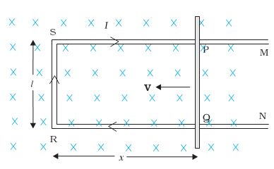
FIGURE 6.10 The arm PQ is moved to the left side, thus decreasing the area of the rectangular loop. This movement induces a current I as shown.

The rod PQ is moved towards the left with a constant velocity v as shown in the figure. Assume that there is no loss of energy due to friction. PQRS forms a closed circuit enclosing an area that changes as PQ moves. It is placed in a uniform magnetic field B which is perpendicular to the plane of this system. If the length RQ = x and RS = l, the magnetic flux \(% MathType!MTEF!2!1!+- % feaagKart1ev2aaatCvAUfeBSjuyZL2yd9gzLbvyNv2CaerbuLwBLn % hiov2DGi1BTfMBaeXatLxBI9gBaerbd9wDYLwzYbItLDharqqtubsr % 4rNCHbGeaGqiVu0Je9sqqrpepC0xbbL8F4rqqrFfpeea0xe9Lq-Jc9 % vqaqpepm0xbba9pwe9Q8fs0-yqaqpepae9pg0FirpepeKkFr0xfr-x % fr-xb9adbaqaaeGaciGaaiaabeqaamaabaabaaGcbaGaeuOPdy0aaS % baaSqaaiaadkeaaeqaaaaa!3863! {\Phi _B}\) enclosed by the loop PQRS will be 

\(% MathType!MTEF!2!1!+- % feaagKart1ev2aaatCvAUfeBSjuyZL2yd9gzLbvyNv2CaerbuLwBLn % hiov2DGi1BTfMBaeXatLxBI9gBaerbd9wDYLwzYbItLDharqqtubsr % 4rNCHbGeaGqiVu0Je9sqqrpepC0xbbL8F4rqqrFfpeea0xe9Lq-Jc9 % vqaqpepm0xbba9pwe9Q8fs0-yqaqpepae9pg0FirpepeKkFr0xfr-x % fr-xb9adbaqaaeGaciGaaiaabeqaamaabaabaaGcbaGaeuOPdy0aaS % baaSqaaiaadkeaaeqaaOGaeyypa0JaamOqaiaadYgacaWG4baaaa!3C28! {\Phi _B} = Blx\)

Since x is changing with time, the rate of change of flux \(% MathType!MTEF!2!1!+- % feaagKart1ev2aaatCvAUfeBSjuyZL2yd9gzLbvyNv2CaerbuLwBLn % hiov2DGi1BTfMBaeXatLxBI9gBaerbd9wDYLwzYbItLDharqqtubsr % 4rNCHbGeaGqiVu0Je9sqqrpepC0xbbL8F4rqqrFfpeea0xe9Lq-Jc9 % vqaqpepm0xbba9pwe9Q8fs0-yqaqpepae9pg0FirpepeKkFr0xfr-x % fr-xb9adbaqaaeGaciGaaiaabeqaamaabaabaaGcbaGaeuOPdy0aaS % baaSqaaiaadkeaaeqaaaaa!3863! {\Phi _B}\) will induce an emf given by:

\(% MathType!MTEF!2!1!+- % feaagKart1ev2aaatCvAUfeBSjuyZL2yd9gzLbvyNv2CaerbuLwBLn % hiov2DGi1BTfMBaeXatLxBI9gBaerbd9wDYLwzYbItLDharqqtubsr % 4rNCHbGeaGqiVu0Je9sqqrpepC0xbbL8F4rqqrFfpeea0xe9Lq-Jc9 % vqaqpepm0xbba9pwe9Q8fs0-yqaqpepae9pg0FirpepeKkFr0xfr-x % fr-xb9adbaqaaeGaciGaaiaabeqaamaabaabaaGceaqabeaacqaH1o % qzcqGH9aqpdaWcaaqaaiabgkHiTiaadsgacqqHMoGrdaWgaaWcbaGa % amOqaaqabaaakeaacaWGKbGaamiDaaaacqGH9aqpcqGHsisldaWcaa % qaaiaadsgaaeaacaWGKbGaamiDaaaadaqadaqaaiaadkeacaWGSbGa % amiEaaGaayjkaiaawMcaaaqaaiabg2da9iabgkHiTiaadkeacaWGSb % WaaSaaaeaacaWGKbGaamiEaaqaaiaadsgacaWG0baaaiabg2da9iaa % dkeacaWGSbGaamODaiaaykW7caaMc8UaaGPaVlaaykW7caaMc8UaaG % PaVlaaykW7caaMc8UaaGPaVlaaykW7caaMc8UaaGPaVlaaykW7caaM % c8UaaGPaVlaaykW7caaMc8UaaGPaVlaaykW7caaMc8UaaGPaVlaayk % W7caaMc8UaaGPaVlaaykW7caaMc8UaaGPaVlaaykW7caaMc8UaaGPa % VlaaykW7caaMc8UaaGPaVlaaykW7caaMc8UaaGPaVpaabmaabaGaaG % Onaiaac6cacaaI1aaacaGLOaGaayzkaaaaaaa!8E77! \begin{array}{l} \varepsilon = \frac{{ - d{\Phi _B}}}{{dt}} = - \frac{d}{{dt}}\left( {Blx} \right)\\ = - Bl\frac{{dx}}{{dt}} = Blv\,\,\,\,\,\,\,\,\,\,\,\,\,\,\,\,\,\,\,\,\,\,\,\,\,\,\,\,\,\,\,\,\,\,\,\,\left( {6.5} \right) \end{array}\)

where we have used dx/dt = –v which is the speed of the conductor PQ. The induced emf Blv is called motional emf. Thus, we are able to produce induced emf by moving a conductor instead of varying the magnetic field, that is, by changing the magnetic flux enclosed by the circuit.

It is also possible to explain the motional emf expression in Eq. (6.5) by invoking the Lorentz force acting on the free charge carriers of conductor PQ. Consider any arbitrary charge q in the conductor PQ. When the rod moves with speed \(v\), the charge will also be moving with speed \(v\) in the magnetic field B. The Lorentz force on this charge is q\(v\)B in magnitude, and its direction is towards Q. All charges experience the same force, in magnitude and direction, irrespective of their position in the rod PQ. The work done in moving the charge from P to Q is,

W = q\(v\)Bl

Since emf is the work done per unit charge,

\(% MathType!MTEF!2!1!+- % feaagKart1ev2aaatCvAUfeBSjuyZL2yd9gzLbvyNv2CaerbuLwBLn % hiov2DGi1BTfMBaeXatLxBI9gBaerbd9wDYLwzYbItLDharqqtubsr % 4rNCHbGeaGqiVu0Je9sqqrpepC0xbbL8F4rqqrFfpeea0xe9Lq-Jc9 % vqaqpepm0xbba9pwe9Q8fs0-yqaqpepae9pg0FirpepeKkFr0xfr-x % fr-xb9adbaqaaeGaciGaaiaabeqaamaabaabaaGceaqabeaacqaH1o % qzcqGH9aqpdaWcaaqaaiaadEfaaeaacaWGXbaaaaqaaiabg2da9iaa % dkeacaWGSbGaamODaaaaaa!3E45! \begin{array}{l} \varepsilon = \frac{W}{q}\\ = Blv \end{array}\)

This equation gives emf induced across the rod PQ and is identical to Eq. (6.5). We stress that our presentation is not wholly rigorous. But it does help us to understand the basis of Faraday’s law when the conductor is moving in a uniform and time-independent magnetic field.

On the other hand, it is not obvious how an emf is induced when a conductor is stationary and the magnetic field is changing – a fact which Faraday verified by numerous experiments. In the case of a stationary conductor, the force on its charges is given by

F = q (E + v \(\times\) B) = qE                                                                      (6.6)

since v = 0. Thus, any force on the charge must arise from the electric field term E alone. Therefore, to explain the existence of induced emf or induced current, we must assume that a time-varying magnetic field generates an electric field. However, we hasten to add that electric fields produced by static electric charges have properties different from those produced by time-varying magnetic fields. In Chapter 4, we learnt that charges in motion (current) can exert force/torque on a stationary magnet. Conversely, a bar magnet in motion (or more generally, a changing magnetic field) can exert a force on the stationary charge. This is the fundamental significance of the Faraday’s discovery. Electricity and magnetism are related.

EXAMPLE 6

A metallic rod of 1 m length is rotated with a frequency of 50 rev/s, with one end hinged at the centre and the other end at the circumference of a circular metallic ring of radius 1 m, about an axis passing through the centre and perpendicular to the plane of the ring (Fig. 6.11). A constant and uniform magnetic field of 1 T parallel to the axis is present everywhere. What is the emf between the centre and the metallic ring?

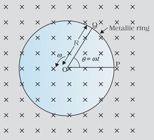
Fig. 6.11

SOLUTION

Method I

As the rod is rotated, free electrons in the rod move towards the outer end due to Lorentz force and get distributed over the ring. Thus, the resulting separation of charges produces an emf across the ends of the rod. At a certain value of emf, there is no more flow of electrons and a steady state is reached. Using Eq. (6.5), the magnitude of the emf generated across a length dr of the rod as it moves at right angles to the magnetic field is given by

d\(% MathType!MTEF!2!1!+- % feaagKart1ev2aaatCvAUfeBSjuyZL2yd9gzLbvyNv2CaerbuLwBLn % hiov2DGi1BTfMBaeXatLxBI9gBaerbd9wDYLwzYbItLDharqqtubsr % 4rNCHbGeaGqiVu0Je9sqqrpepC0xbbL8F4rqqrFfpeea0xe9Lq-Jc9 % vqaqpepm0xbba9pwe9Q8fs0-yqaqpepae9pg0FirpepeKkFr0xfr-x % fr-xb9adbaqaaeGaciGaaiaabeqaamaabaabaaGcbaGaeqyTduMaey % ypa0JaamOqaiaadAhaaaa!3A65! \varepsilon = Bv\) dr . Hence,

\(% MathType!MTEF!2!1!+- % feaagKart1ev2aaatCvAUfeBSjuyZL2yd9gzLbvyNv2CaerbuLwBLn % hiov2DGi1BTfMBaeXatLxBI9gBaerbd9wDYLwzYbItLDharqqtubsr % 4rNCHbGeaGqiVu0Je9sqqrpepC0xbbL8F4rqqrFfpeea0xe9Lq-Jc9 % vqaqpepm0xbba9pwe9Q8fs0-yqaqpepae9pg0FirpepeKkFr0xfr-x % fr-xb9adbaqaaeGaciGaaiaabeqaamaabaabaaGcbiqaaaWacqaH1o % qzcqGH9aqpdaWdbaqaaiaadsgacqaH1oqzcqGH9aqpdaWdXbqaaiaa % dkeacaWG2bGaamizaiaadkhaaSqaaiaaicdaaeaacaWGsbaaniabgU % IiYdGccqGH9aqpaSqabeqaniabgUIiYdGcdaWdXbqaaiaadkeacqaH % jpWDcaWGYbGaamizaiaadkhaaSqaaiaaicdaaeaacaWGsbaaniabgU % IiYdGccqGH9aqpdaWcaaqaaiaadkeacqaHjpWDcaWGsbWaaWbaaSqa % beaacaaIYaaaaaGcbaGaaGOmaaaaaaa!568F! \varepsilon = \int {d\varepsilon = \int\limits_0^R {Bvdr} = } \int\limits_0^R {B\omega rdr} = \frac{{B\omega {R^2}}}{2}\)

Note that we have used v = \(% MathType!MTEF!2!1!+- % feaagKart1ev2aaatCvAUfeBSjuyZL2yd9gzLbvyNv2CaerbuLwBLn % hiov2DGi1BTfMBaeXatLxBI9gBaerbd9wDYLwzYbItLDharqqtubsr % 4rNCHbGeaGqiVu0Je9sqqrpepC0xbbL8F4rqqrFfpeea0xe9Lq-Jc9 % vqaqpepm0xbba9pwe9Q8fs0-yqaqpepae9pg0FirpepeKkFr0xfr-x % fr-xb9adbaqaaeGaciGaaiaabeqaamaabaabaaGcbaGaeqyYdChaaa!37C3! \omega \) r. This gives

\(% MathType!MTEF!2!1!+- % feaagKart1ev2aaatCvAUfeBSjuyZL2yd9gzLbvyNv2CaerbuLwBLn % hiov2DGi1BTfMBaeXatLxBI9gBaerbd9wDYLwzYbItLDharqqtubsr % 4rNCHbGeaGqiVu0Je9sqqrpepC0xbbL8F4rqqrFfpeea0xe9Lq-Jc9 % vqaqpepm0xbba9pwe9Q8fs0-yqaqpepae9pg0FirpepeKkFr0xfr-x % fr-xb9adbaqaaeGaciGaaiaabeqaamaabaabaaGceiqabeaaamqaai % abew7aLjabg2da9maalaaabaGaaGymaaqaaiaaikdaaaGaey41aqRa % aGymaiaac6cacaaIWaGaey41aqRaaGOmaiabec8aWjabgEna0kaaiw % dacaaIWaGaey41aq7aaeWaaeaacaaIXaWaaWbaaSqabeaacaaIYaaa % aaGccaGLOaGaayzkaaaabaGaeyypa0JaaGymaiaaiwdacaaI3aGaam % Ovaaaaaa!4FFF! \begin{array}{l} \varepsilon = \frac{1}{2} \times 1.0 \times 2\pi \times 50 \times \left( {{1^2}} \right)\\ = 157V \end{array}\)

Method II

To calculate the emf, we can imagine a closed loop OPQ in which point O and P are connected with a resistor R and OQ is the rotating rod. The potential difference across the resistor is then equal to the induced emf and equals B × (rate of change of area of loop). If \(\theta\) is the angle between the rod and the radius of the circle at P at time t, the area of the sector OPQ is given by 

\(% MathType!MTEF!2!1!+- % feaagKart1ev2aaatCvAUfeBSjuyZL2yd9gzLbvyNv2CaerbuLwBLn % hiov2DGi1BTfMBaeXatLxBI9gBaerbd9wDYLwzYbItLDharqqtubsr % 4rNCHbGeaGqiVu0Je9sqqrpepC0xbbL8F4rqqrFfpeea0xe9Lq-Jc9 % vqaqpepm0xbba9pwe9Q8fs0-yqaqpepae9pg0FirpepeKkFr0xfr-x % fr-xb9adbaqaaeGaciGaaiaabeqaamaabaabaaGcbiqaaaWacqaHap % aCcaWGsbWaaWbaaSqabeaacaaIYaaaaOGaey41aq7aaSaaaeaacqaH % 4oqCaeaacaaIYaGaeqiWdahaaiabg2da9maalaaabaGaaGymaaqaai % aaikdaaaGaamOuamaaCaaaleqabaGaaGOmaaaakiabeI7aXbaa!45E6! \pi {R^2} \times \frac{\theta }{{2\pi }} = \frac{1}{2}{R^2}\theta \)

where R is the radius of the circle. Hence, the induced emf is

\(% MathType!MTEF!2!1!+- % feaagKart1ev2aaatCvAUfeBSjuyZL2yd9gzLbvyNv2CaerbuLwBLn % hiov2DGi1BTfMBaeXatLxBI9gBaerbd9wDYLwzYbItLDharqqtubsr % 4rNCHbGeaGqiVu0Je9sqqrpepC0xbbL8F4rqqrFfpeea0xe9Lq-Jc9 % vqaqpepm0xbba9pwe9Q8fs0-yqaqpepae9pg0FirpepeKkFr0xfr-x % fr-xb9adbaqaaeGaciGaaiaabeqaamaabaabaaGceiqabeaaamqaai % abew7aLjabg2da9iaadkeacqGHxdaTdaWcaaqaaiaadsgaaeaacaWG % KbGaamiDaaaadaWadaqaamaalaaabaGaaGymaaqaaiaaikdaaaGaam % OuamaaCaaaleqabaGaaGOmaaaakiabeI7aXbGaay5waiaaw2faaiab % g2da9maalaaabaGaaGymaaqaaiaaikdaaaGaamOqaiaadkfadaahaa % WcbeqaaiaaikdaaaGcdaWcaaqaaiaadsgacqaH4oqCaeaacaWGKbGa % amiDaaaacqGH9aqpdaWcaaqaaiaadkeacqaHjpWDcaWGsbWaaWbaaS % qabeaacaaIYaaaaaGcbaGaaGOmaaaaaeaadaWadaqaaiaad6eacaWG % VbGaamiDaiaadwgacaaMc8UaaiOoaiaaykW7daWcaaqaaiaadsgacq % aH4oqCaeaacaWGKbGaamiDaaaacqGH9aqpcqaHjpWDcqGH9aqpcaaI % YaGaeqiWdaNaamODaaGaay5waiaaw2faaaaaaa!6A8F! \begin{array}{l} \varepsilon = B \times \frac{d}{{dt}}\left[ {\frac{1}{2}{R^2}\theta } \right] = \frac{1}{2}B{R^2}\frac{{d\theta }}{{dt}} = \frac{{B\omega {R^2}}}{2}\\ \left[ {Note\,:\,\frac{{d\theta }}{{dt}} = \omega = 2\pi v} \right] \end{array}\)

This expression is identical to the expression obtained by Method I and we get the same value of \(% MathType!MTEF!2!1!+- % feaagKart1ev2aaatCvAUfeBSjuyZL2yd9gzLbvyNv2CaerbuLwBLn % hiov2DGi1BTfMBaeXatLxBI9gBaerbd9wDYLwzYbItLDharqqtubsr % 4rNCHbGeaGqiVu0Je9sqqrpepC0xbbL8F4rqqrFfpeea0xe9Lq-Jc9 % vqaqpepm0xbba9pwe9Q8fs0-yqaqpepae9pg0FirpepeKkFr0xfr-x % fr-xb9adbaqaaeGaciGaaiaabeqaamaabaabaaGcbiqaaaWacqaH1o % qzaaa!37A3! \varepsilon \).

EXAMPLE 7

A wheel with 10 metallic spokes each 0.5 m long is rotated with a speed of 120 rev/min in a plane normal to the horizontal component of earth’s magnetic field HE at a place. If HE = 0.4 G at the place, what is the induced emf between the axle and the rim of the wheel? Note that 1 G = 10^–4 T.

SOLUTION

Induced emf = (1/2) \(% MathType!MTEF!2!1!+- % feaagKart1ev2aaatCvAUfeBSjuyZL2yd9gzLbvyNv2CaerbuLwBLn % hiov2DGi1BTfMBaeXatLxBI9gBaerbd9wDYLwzYbItLDharqqtubsr % 4rNCHbGeaGqiVu0Je9sqqrpepC0xbbL8F4rqqrFfpeea0xe9Lq-Jc9 % vqaqpepm0xbba9pwe9Q8fs0-yqaqpepae9pg0FirpepeKkFr0xfr-x % fr-xb9adbaqaaeGaciGaaiaabeqaamaabaabaaGcbiqaaaWacqaHjp % WDaaa!37C9! \omega \) B R²

= (1/2) × 4\(\pi\) × 0.4 × 10^–4 × (0.5)²

= 6.28 × 10^–5 V

The number of spokes is immaterial because the emf’s across the spokes are in parallel.