-
Introduction to Inductance
Introduction to Inductance
An electric current can be induced in a coil by flux change produced by another coil in its vicinity or flux change produced by the same coil. These two situations are described separately in the next two sub-sections. However, in both the cases, the flux through a coil is proportional to the current. That is, \(% MathType!MTEF!2!1!+- % feaagKart1ev2aaatCvAUfeBSjuyZL2yd9gzLbvyNv2CaerbuLwBLn % hiov2DGi1BTfMBaeXatLxBI9gBaerbd9wDYLwzYbItLDharqqtubsr % 4rNCHbGeaGqiVu0Je9sqqrpepC0xbbL8F4rqqrFfpeea0xe9Lq-Jc9 % vqaqpepm0xbba9pwe9Q8fs0-yqaqpepae9pg0FirpepeKkFr0xfr-x % fr-xb9adbaqaaeGaciGaaiaabeqaamaabaabaaGcbiqaaaWacqqHMo % GrdaWgaaWcbaGaamOqaaqabaGccqaHXoqyaaa!3A12! {\Phi _B}\alpha \) I.
Further, if the geometry of the coil does not vary with time then,
\(% MathType!MTEF!2!1!+- % feaagKart1ev2aaatCvAUfeBSjuyZL2yd9gzLbvyNv2CaerbuLwBLn % hiov2DGi1BTfMBaeXatLxBI9gBaerbd9wDYLwzYbItLDharqqtubsr % 4rNCHbGeaGqiVu0Je9sqqrpepC0xbbL8F4rqqrFfpeea0xe9Lq-Jc9 % vqaqpepm0xbba9pwe9Q8fs0-yqaqpepae9pg0FirpepeKkFr0xfr-x % fr-xb9adbaqaaeGaciGaaiaabeqaamaabaabaaGcbiqaaaWadaWcaa % qaceaaamGaamizaiabfA6agnaaBaaaleaacaWGcbaabeaaaOqaaiaa % dsgacaWG0baaaabaaaaaaaaapeGaeyyhIu7aaSaaaeaacaWGKbGaam % ysaaqaaiaadsgacaWG0baaaaaa!409D! \frac{{d{\Phi _B}}}{{dt}} \propto \frac{{dI}}{{dt}}\)
For a closely wound coil of N turns, the same magnetic flux is linked with all the turns. When the flux \(% MathType!MTEF!2!1!+- % feaagKart1ev2aaatCvAUfeBSjuyZL2yd9gzLbvyNv2CaerbuLwBLn % hiov2DGi1BTfMBaeXatLxBI9gBaerbd9wDYLwzYbItLDharqqtubsr % 4rNCHbGeaGqiVu0Je9sqqrpepC0xbbL8F4rqqrFfpeea0xe9Lq-Jc9 % vqaqpepm0xbba9pwe9Q8fs0-yqaqpepae9pg0FirpepeKkFr0xfr-x % fr-xb9adbaqaaeGaciGaaiaabeqaamaabaabaaGcbaGaeuOPdy0aaS % baaSqaaiaadkeaaeqaaaaa!3863! {{\Phi _B}}\) through the coil changes, each turn contributes to the induced emf. Therefore, a term called flux linkage is used which is equal to N\(% MathType!MTEF!2!1!+- % feaagKart1ev2aaatCvAUfeBSjuyZL2yd9gzLbvyNv2CaerbuLwBLn % hiov2DGi1BTfMBaeXatLxBI9gBaerbd9wDYLwzYbItLDharqqtubsr % 4rNCHbGeaGqiVu0Je9sqqrpepC0xbbL8F4rqqrFfpeea0xe9Lq-Jc9 % vqaqpepm0xbba9pwe9Q8fs0-yqaqpepae9pg0FirpepeKkFr0xfr-x % fr-xb9adbaqaaeGaciGaaiaabeqaamaabaabaaGcbaGaeuOPdy0aaS % baaSqaaiaadkeaaeqaaaaa!3863! {{\Phi _B}}\) for a closely wound coil and in such a case
N \(% MathType!MTEF!2!1!+- % feaagKart1ev2aaatCvAUfeBSjuyZL2yd9gzLbvyNv2CaerbuLwBLn % hiov2DGi1BTfMBaeXatLxBI9gBaerbd9wDYLwzYbItLDharqqtubsr % 4rNCHbGeaGqiVu0Je9sqqrpepC0xbbL8F4rqqrFfpeea0xe9Lq-Jc9 % vqaqpepm0xbba9pwe9Q8fs0-yqaqpepae9pg0FirpepeKkFr0xfr-x % fr-xb9adbaqaaeGaciGaaiaabeqaamaabaabaaGcbiqaaaWaqaaaaa % aaaaWdbiaaygW7caaMb8UaaGzaVlaaygW7cqqHMoGrdaWgaaWcbaGa % amOqaaqabaGccqGHDisTcaWGjbaaaa!4109! {\Phi _B} \propto I\)
The constant of proportionality, in this relation, is called inductance. We shall see that inductance depends only on the geometry of the coil
and intrinsic material properties. This aspect is akin to capacitance which for a parallel plate capacitor depends on the plate area and plate separation (geometry) and the dielectric constant K of the intervening medium (intrinsic material property).
Inductance is a scalar quantity. It has the dimensions of [M L2 T–2 A–2] given by the dimensions of flux divided by the dimensions of current. The SI unit of inductance is henry and is denoted by H. It is named in honour of Joseph Henry who discovered electromagnetic induction in USA, independently of Faraday in England.
-
Mutual Inductance
Mutual Inductance
Consider Fig. 6.15 which shows two long co-axial solenoids each of length l.
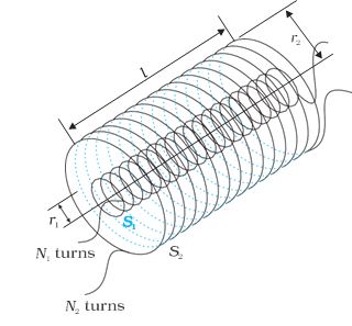
FIGURE 6.15 Two long coaxial solenoids of same length l.
We denote the radius of the inner solenoid S1 by r1 and the number of turns per unit length by n1. The corresponding quantities for the outer solenoid S2 are r2 and n2, respectively. Let N1 and N2 be the total number of turns of coils S1 and S2, respectively.
When a current I2 is set up through S2, it in turn sets up a magnetic flux through S1. Let us denote it by \(% MathType!MTEF!2!1!+- % feaagKart1ev2aaatCvAUfeBSjuyZL2yd9gzLbvyNv2CaerbuLwBLn % hiov2DGi1BTfMBaeXatLxBI9gBaerbd9wDYLwzYbItLDharqqtubsr % 4rNCHbGeaGqiVu0Je9sqqrpepC0xbbL8F4rqqrFfpeea0xe9Lq-Jc9 % vqaqpepm0xbba9pwe9Q8fs0-yqaqpepae9pg0FirpepeKkFr0xfr-x % fr-xb9adbaqaaeGaciGaaiaabeqaamaabaabaaGcbaaeaaaaaaaaa8 % qacqqHMoGraaa!3790! \Phi \)1. The corresponding flux linkage with solenoid S1 is
\(% MathType!MTEF!2!1!+- % feaagKart1ev2aaatCvAUfeBSjuyZL2yd9gzLbvyNv2CaerbuLwBLn % hiov2DGi1BTfMBaeXatLxBI9gBaerbd9wDYLwzYbItLDharqqtubsr % 4rNCHbGeaGqiVu0Je9sqqrpepC0xbbL8F4rqqrFfpeea0xe9Lq-Jc9 % vqaqpepm0xbba9pwe9Q8fs0-yqaqpepae9pg0FirpepeKkFr0xfr-x % fr-xb9adbaqaaeGaciGaaiaabeqaamaabaabaaGcbaGaamOtamaaBa % aaleaacaaIXaaabeaakiabfA6agnaaBaaaleaacaaIXaaabeaakiab % g2da9iaad2eadaWgaaWcbaGaaGymaiaaikdaaeqaaOGaamysamaaBa % aaleaacaaIYaaabeaaaaa!3F60! {N_1}{\Phi _1} = {M_{12}}{I_2}\) (6.9)
M12 is called the mutual inductance of solenoid S1 with respect to solenoid S2. It is also referred to as the coefficient of mutual induction.
For these simple co-axial solenoids it is possible to calculate M12. The magnetic field due to the current I2 in S2 is \(\mu\)0n2I2. The resulting flux linkage with coil S1 is,
\(% MathType!MTEF!2!1!+- % feaagKart1ev2aaatCvAUfeBSjuyZL2yd9gzLbvyNv2CaerbuLwBLn % hiov2DGi1BTfMBaeXatLxBI9gBaerbd9wDYLwzYbItLDharqqtubsr % 4rNCHbGeaGqiVu0Je9sqqrpepC0xbbL8F4rqqrFfpeea0xe9Lq-Jc9 % vqaqpepm0xbba9pwe9Q8fs0-yqaqpepae9pg0FirpepeKkFr0xfr-x % fr-xb9adbaqaaeGaciGaaiaabeqaamaabaabaaGceaqabeaacaWGob % WaaSbaaSqaaiaaigdaaeqaaOGaeuOPdy0aaSbaaSqaaiaaigdaaeqa % aOGaeyypa0ZaaeWaaeaacaWGUbWaaSbaaSqaaiaaigdaaeqaaOGaam % iBaaGaayjkaiaawMcaamaabmaabaGaeqiWdaNaamOCamaaDaaaleaa % caaIXaaabaGaaGOmaaaaaOGaayjkaiaawMcaamaabmaabaGaeqiVd0 % 2aaSbaaSqaaiaaicdaaeqaaOGaamOBamaaBaaaleaacaaIYaaabeaa % kiaadYgadaWgaaWcbaGaaGOmaaqabaaakiaawIcacaGLPaaaaeaacq % GH9aqpcqaH8oqBdaWgaaWcbaGaaGimaaqabaGccaWGUbWaaSbaaSqa % aiaaigdaaeqaaOGaamOBamaaBaaaleaacaaIYaaabeaakiabec8aWj % aadkhadaqhaaWcbaGaaGymaaqaaiaaigdaaaGccaWGSbGaamysamaa % BaaaleaacaaIYaaabeaakiaaykW7caaMc8UaaGPaVlaaykW7caaMc8 % UaaGPaVlaaykW7caaMc8UaaGPaVlaaykW7caaMc8UaaGPaVlaaykW7 % caaMc8UaaGPaVlaaykW7caaMc8UaaGPaVlaaykW7caaMc8UaaGPaVl % aaykW7caaMc8UaaGPaVlaaykW7caaMc8UaaGPaVlaaykW7caaMc8Ua % aGPaVlaaykW7caaMc8UaaGPaVlaaykW7caaMc8UaaGPaVlaaykW7ca % aMc8UaaGPaVlaaykW7caaMc8+aaeWaaeaacaaI2aGaaiOlaiaaigda % caaIWaaacaGLOaGaayzkaaaaaaa!9FAC! \begin{array}{l} {N_1}{\Phi _1} = \left( {{n_1}l} \right)\left( {\pi r_1^2} \right)\left( {{\mu _0}{n_2}{l_2}} \right)\\ = {\mu _0}{n_1}{n_2}\pi r_1^1l{I_2}\,\,\,\,\,\,\,\,\,\,\,\,\,\,\,\,\,\,\,\,\,\,\,\,\,\,\,\,\,\,\,\,\,\,\,\,\,\,\,\,\,\left( {6.10} \right) \end{array}\) (6.10)
where n1l is the total number of turns in solenoid S1. Thus, from Eq. (6.9) and Eq. (6.10),
\(% MathType!MTEF!2!1!+- % feaagKart1ev2aaatCvAUfeBSjuyZL2yd9gzLbvyNv2CaerbuLwBLn % hiov2DGi1BTfMBaeXatLxBI9gBaerbd9wDYLwzYbItLDharqqtubsr % 4rNCHbGeaGqiVu0Je9sqqrpepC0xbbL8F4rqqrFfpeea0xe9Lq-Jc9 % vqaqpepm0xbba9pwe9Q8fs0-yqaqpepae9pg0FirpepeKkFr0xfr-x % fr-xb9adbaqaaeGaciGaaiaabeqaamaabaabaaGcbaGaamytamaaBa % aaleaacaaIXaGaaGOmaaqabaGccqGH9aqpcqaH8oqBdaWgaaWcbaGa % aGimaaqabaGccaWGUbWaaSbaaSqaaiaaigdaaeqaaOGaamOBamaaBa % aaleaacaaIYaaabeaakiabec8aWjaadkhadaqhaaWcbaGaaGymaaqa % aiaaikdaaaGccaWGSbaaaa!453D! {M_{12}} = {\mu _0}{n_1}{n_2}\pi r_1^2l\) (6.11)
Note that we neglected the edge effects and considered the magnetic field \(\mu\)0n2I2 to be uniform throughout the length and width of the solenoid S2. This is a good approximation keeping in mind that the solenoid is long, implying l >> r2.
We now consider the reverse case. A current I1 is passed through the solenoid S1 and the flux linkage with coil S2 is,
\(% MathType!MTEF!2!1!+- % feaagKart1ev2aaatCvAUfeBSjuyZL2yd9gzLbvyNv2CaerbuLwBLn % hiov2DGi1BTfMBaeXatLxBI9gBaerbd9wDYLwzYbItLDharqqtubsr % 4rNCHbGeaGqiVu0Je9sqqrpepC0xbbL8F4rqqrFfpeea0xe9Lq-Jc9 % vqaqpepm0xbba9pwe9Q8fs0-yqaqpepae9pg0FirpepeKkFr0xfr-x % fr-xb9adbaqaaeGaciGaaiaabeqaamaabaabaaGcbaGaamOtamaaBa % aaleaacaaIYaaabeaakiabfA6agnaaBaaaleaacaaIYaaabeaakiab % g2da9iaad2eadaWgaaWcbaGaaGOmaiaaigdaaeqaaOGaamysamaaBa % aaleaacaaIXaaabeaaaaa!3F61! {N_2}{\Phi _2} = {M_{21}}{I_1}\) (6.12)
M21 is called the mutual inductance of solenoid S2 with respect to solenoid S1.
The flux due to the current I1 in S1 can be assumed to be confined solely inside S1 since the solenoids are very long. Thus, flux linkage with solenoid S2 is
\(% MathType!MTEF!2!1!+- % feaagKart1ev2aaatCvAUfeBSjuyZL2yd9gzLbvyNv2CaerbuLwBLn % hiov2DGi1BTfMBaeXatLxBI9gBaerbd9wDYLwzYbItLDharqqtubsr % 4rNCHbGeaGqiVu0Je9sqqrpepC0xbbL8F4rqqrFfpeea0xe9Lq-Jc9 % vqaqpepm0xbba9pwe9Q8fs0-yqaqpepae9pg0FirpepeKkFr0xfr-x % fr-xb9adbaqaaeGaciGaaiaabeqaamaabaabaaGcbaGaamOtamaaBa % aaleaacaaIYaaabeaakiabfA6agnaaBaaaleaacaaIYaaabeaakiab % g2da9maabmaabaGaamOBamaaBaaaleaacaaIXaaabeaakiaadYgaai % aawIcacaGLPaaadaqadaqaaiabec8aWjaadkhadaqhaaWcbaGaaGym % aaqaaiaaikdaaaaakiaawIcacaGLPaaadaqadaqaaiabeY7aTnaaBa % aaleaacaaIWaaabeaakiaad6gadaWgaaWcbaGaaGymaaqabaGccaWG % jbWaaSbaaSqaaiaaigdaaeqaaaGccaGLOaGaayzkaaaaaa!4D48! {N_2}{\Phi _2} = \left( {{n_1}l} \right)\left( {\pi r_1^2} \right)\left( {{\mu _0}{n_1}{I_1}} \right)\)
where n2l is the total number of turns of S2. From Eq. (6.12),
\(% MathType!MTEF!2!1!+- % feaagKart1ev2aaatCvAUfeBSjuyZL2yd9gzLbvyNv2CaerbuLwBLn % hiov2DGi1BTfMBaeXatLxBI9gBaerbd9wDYLwzYbItLDharqqtubsr % 4rNCHbGeaGqiVu0Je9sqqrpepC0xbbL8F4rqqrFfpeea0xe9Lq-Jc9 % vqaqpepm0xbba9pwe9Q8fs0-yqaqpepae9pg0FirpepeKkFr0xfr-x % fr-xb9adbaqaaeGaciGaaiaabeqaamaabaabaaGcbaGaamytamaaBa % aaleaacaaIYaGaaGymaaqabaGccqGH9aqpcqaH8oqBdaWgaaWcbaGa % aGimaaqabaGccaWGUbWaaSbaaSqaaiaaigdaaeqaaOGaamOBamaaBa % aaleaacaaIYaaabeaakiabec8aWjaadkhadaqhaaWcbaGaaGymaaqa % aiaaikdaaaGccaWGSbaaaa!453D! {M_{21}} = {\mu _0}{n_1}{n_2}\pi r_1^2l\) (6.13)
Using Eq. (6.11) and Eq. (6.12), we get
\(% MathType!MTEF!2!1!+- % feaagKart1ev2aaatCvAUfeBSjuyZL2yd9gzLbvyNv2CaerbuLwBLn % hiov2DGi1BTfMBaeXatLxBI9gBaerbd9wDYLwzYbItLDharqqtubsr % 4rNCHbGeaGqiVu0Je9sqqrpepC0xbbL8F4rqqrFfpeea0xe9Lq-Jc9 % vqaqpepm0xbba9pwe9Q8fs0-yqaqpepae9pg0FirpepeKkFr0xfr-x % fr-xb9adbaqaaeGaciGaaiaabeqaamaabaabaaGcbaGaamytamaaBa % aaleaacaaIXaGaaGOmaaqabaGccqGH9aqpcaWGnbWaaSbaaSqaaiaa % ikdacaaIXaaabeaakiabg2da9iaad2eadaqadaqaaiaadohacaWGHb % GaamyEaaGaayjkaiaawMcaaaaa!4237! {M_{12}} = {M_{21}} = M\left( {say} \right)\) (6.14)
We have demonstrated this equality for long co-axial solenoids. However, the relation is far more general. Note that if the inner solenoid was much shorter than (and placed well inside) the outer solenoid, then we could still have calculated the flux linkage N1\(% MathType!MTEF!2!1!+- % feaagKart1ev2aaatCvAUfeBSjuyZL2yd9gzLbvyNv2CaerbuLwBLn % hiov2DGi1BTfMBaeXatLxBI9gBaerbd9wDYLwzYbItLDharqqtubsr % 4rNCHbGeaGqiVu0Je9sqqrpepC0xbbL8F4rqqrFfpeea0xe9Lq-Jc9 % vqaqpepm0xbba9pwe9Q8fs0-yqaqpepae9pg0FirpepeKkFr0xfr-x % fr-xb9adbaqaaeGaciGaaiaabeqaamaabaabaaGcbaGaeuOPdyeaaa!3770! \Phi \)1 because the inner solenoid is effectively immersed in a uniform magnetic field due to the outer solenoid. In this case, the calculation of M12 would be easy. However, it would be extremely difficult to calculate the flux linkage with the outer solenoid as the magnetic field due to the inner solenoid would vary across the length as well as cross section of the outer solenoid. Therefore, the calculation of M21 would also be extremely difficult in this case. The equality M12=M21 is very useful in such situations.
We explained the above example with air as the medium within the solenoids. Instead, if a medium of relative permeability \(\mu\)r had been present, the mutual inductance would be
\(% MathType!MTEF!2!1!+- % feaagKart1ev2aaatCvAUfeBSjuyZL2yd9gzLbvyNv2CaerbuLwBLn % hiov2DGi1BTfMBaeXatLxBI9gBaerbd9wDYLwzYbItLDharqqtubsr % 4rNCHbGeaGqiVu0Je9sqqrpepC0xbbL8F4rqqrFfpeea0xe9Lq-Jc9 % vqaqpepm0xbba9pwe9Q8fs0-yqaqpepae9pg0FirpepeKkFr0xfr-x % fr-xb9adbaqaaeGaciGaaiaabeqaamaabaabaaGcbaGaamytaiabg2 % da9iabeY7aTnaaBaaaleaacaWGYbaabeaakiabeY7aTnaaBaaaleaa % caaIWaaabeaakiaad6gadaWgaaWcbaGaaGymaaqabaGccaWGUbWaaS % baaSqaaiaaikdaaeqaaOGaeqiWdaNaamOCamaaDaaaleaacaaIXaaa % baGaaGOmaaaakiaadYgaaaa!4673! M = {\mu _r}{\mu _0}{n_1}{n_2}\pi r_1^2l\)
It is also important to know that the mutual inductance of a pair of coils, solenoids, etc., depends on their separation as well as their relative orientation.
EXAMPLE 9
Two concentric circular coils, one of small radius r1 and the other of large radius r2, such that r1 << r2, are placed co-axially with centres coinciding. Obtain the mutual inductance of the arrangement.
Solution
Let a current I2 flow through the outer circular coil. The field at the centre of the coil is B2 = \(\mu\)0I2 / 2r2. Since the other co-axially placed coil has a very small radius, B2 may be considered constant over its cross-sectional area. Hence,
\(% MathType!MTEF!2!1!+- % feaagKart1ev2aaatCvAUfeBSjuyZL2yd9gzLbvyNv2CaerbuLwBLn % hiov2DGi1BTfMBaeXatLxBI9gBaerbd9wDYLwzYbItLDharqqtubsr % 4rNCHbGeaGqiVu0Je9sqqrpepC0xbbL8F4rqqrFfpeea0xe9Lq-Jc9 % vqaqpepm0xbba9pwe9Q8fs0-yqaqpepae9pg0FirpepeKkFr0xfr-x % fr-xb9adbaqaaeGaciGaaiaabeqaamaabaabaaGceaqabeaacqqHMo % GrdaWgaaWcbaGaaGymaaqabaGccqGH9aqpcqaHapaCcaWGYbWaa0ba % aSqaaiaaigdaaeaacaaIYaaaaOGaamOqamaaBaaaleaacaaIYaaabe % aaaOqaaiabg2da9maalaaabaGaeqiVd02aaSbaaSqaaiaaicdaaeqa % aOGaeqiWdaNaamOCamaaDaaaleaacaaIXaaabaGaaGOmaaaaaOqaai % aaikdacaWGYbWaaSbaaSqaaiaaikdaaeqaaaaaaOqaaiaadsfacaWG % ObGaamyDaiaadohacaGGSaaabaGaamytamaaBaaaleaacaaIXaGaaG % OmaaqabaGccqGH9aqpdaWcaaqaaiabeY7aTnaaBaaaleaacaaIWaaa % beaakiabec8aWjaadkhadaqhaaWcbaGaaGymaaqaaiaaikdaaaaake % aacaaIYaGaamOCamaaBaaaleaacaaIYaaabeaaaaaakeaacaWGgbGa % amOCaiaad+gacaWGTbGaaGPaVlaaykW7caaMc8Uaamyraiaadghaca % GGUaWaaeWaaeaacaaI2aGaaiOlaiaaigdacaaI0aaacaGLOaGaayzk % aaaabaGaamytamaaBaaaleaacaaIXaGaaGOmaaqabaGccqGH9aqpca % WGnbWaaSbaaSqaaiaaikdacaaIXaaabeaakiabg2da9maalaaabaGa % eqiVd02aaSbaaSqaaiaaicdaaeqaaOGaeqiWdaNaamOCamaaDaaale % aacaaIXaaabaGaaGOmaaaaaOqaaiaaikdacaWGYbWaaSbaaSqaaiaa % ikdaaeqaaaaaaaaa!7BE6! \begin{array}{l} {\Phi _1} = \pi r_1^2{B_2}\\ = \frac{{{\mu _0}\pi r_1^2}}{{2{r_2}}}\\ Thus,\\ {M_{12}} = \frac{{{\mu _0}\pi r_1^2}}{{2{r_2}}}\\ From\,\,\,Eq.\left( {6.14} \right)\\ {M_{12}} = {M_{21}} = \frac{{{\mu _0}\pi r_1^2}}{{2{r_2}}} \end{array}\)
Note that we calculated M12 from an approximate value of \(% MathType!MTEF!2!1!+- % feaagKart1ev2aaatCvAUfeBSjuyZL2yd9gzLbvyNv2CaerbuLwBLn % hiov2DGi1BTfMBaeXatLxBI9gBaerbd9wDYLwzYbItLDharqqtubsr % 4rNCHbGeaGqiVu0Je9sqqrpepC0xbbL8F4rqqrFfpeea0xe9Lq-Jc9 % vqaqpepm0xbba9pwe9Q8fs0-yqaqpepae9pg0FirpepeKkFr0xfr-x % fr-xb9adbaqaaeGaciGaaiaabeqaamaabaabaaGcbaGaeuOPdyeaaa!3770! \Phi \)1, assuming the magnetic field B2 to be uniform over the area \(% MathType!MTEF!2!1!+- % feaagKart1ev2aaatCvAUfeBSjuyZL2yd9gzLbvyNv2CaerbuLwBLn % hiov2DGi1BTfMBaeXatLxBI9gBaerbd9wDYLwzYbItLDharqqtubsr % 4rNCHbGeaGqiVu0Je9sqqrpepC0xbbL8F4rqqrFfpeea0xe9Lq-Jc9 % vqaqpepm0xbba9pwe9Q8fs0-yqaqpepae9pg0FirpepeKkFr0xfr-x % fr-xb9adbaqaaeGaciGaaiaabeqaamaabaabaaGcbaGaeqiWdaNaam % OCamaaDaaaleaacaaIXaaabaGaaGOmaaaaaaa!3A4E! \pi r_1^2\). However, we can accept this value because r1 << r2.
Now, let us recollect Experiment 6.3 in Section 6.2. In that experiment, emf is induced in coil C1 wherever there was any change in current through coil C2. Let \(% MathType!MTEF!2!1!+- % feaagKart1ev2aaatCvAUfeBSjuyZL2yd9gzLbvyNv2CaerbuLwBLn % hiov2DGi1BTfMBaeXatLxBI9gBaerbd9wDYLwzYbItLDharqqtubsr % 4rNCHbGeaGqiVu0Je9sqqrpepC0xbbL8F4rqqrFfpeea0xe9Lq-Jc9 % vqaqpepm0xbba9pwe9Q8fs0-yqaqpepae9pg0FirpepeKkFr0xfr-x % fr-xb9adbaqaaeGaciGaaiaabeqaamaabaabaaGcbaGaeuOPdyeaaa!3770! \Phi \)1 be the flux through coil C1 (say of N1 turns) when current in coil C2 is I2.
Then, from Eq. (6.9), we have
N1\(% MathType!MTEF!2!1!+- % feaagKart1ev2aaatCvAUfeBSjuyZL2yd9gzLbvyNv2CaerbuLwBLn % hiov2DGi1BTfMBaeXatLxBI9gBaerbd9wDYLwzYbItLDharqqtubsr % 4rNCHbGeaGqiVu0Je9sqqrpepC0xbbL8F4rqqrFfpeea0xe9Lq-Jc9 % vqaqpepm0xbba9pwe9Q8fs0-yqaqpepae9pg0FirpepeKkFr0xfr-x % fr-xb9adbaqaaeGaciGaaiaabeqaamaabaabaaGcbaGaeuOPdyeaaa!3770! \Phi \)1 = MI2
For currents varrying with time,
\(% MathType!MTEF!2!1!+- % feaagKart1ev2aaatCvAUfeBSjuyZL2yd9gzLbvyNv2CaerbuLwBLn % hiov2DGi1BTfMBaeXatLxBI9gBaerbd9wDYLwzYbItLDharqqtubsr % 4rNCHbGeaGqiVu0Je9sqqrpepC0xbbL8F4rqqrFfpeea0xe9Lq-Jc9 % vqaqpepm0xbba9pwe9Q8fs0-yqaqpepae9pg0FirpepeKkFr0xfr-x % fr-xb9adbaqaaeGaciGaaiaabeqaamaabaabaaGcbaWaaSaaaeaaca % WGKbWaaeWaaeaacaWGobWaaSbaaSqaaiaaigdaaeqaaOGaeuOPdy0a % aSbaaSqaaiaaigdaaeqaaaGccaGLOaGaayzkaaaabaGaamizaiaads % haaaGaeyypa0ZaaSaaaeaacaWGKbWaaeWaaeaacaWGnbGaamysamaa % BaaaleaacaaIYaaabeaaaOGaayjkaiaawMcaaaqaaiaadsgacaWG0b % aaaaaa!4685! \frac{{d\left( {{N_1}{\Phi _1}} \right)}}{{dt}} = \frac{{d\left( {M{I_2}} \right)}}{{dt}}\)
Since induced emf in coil C1 is given by
\(% MathType!MTEF!2!1!+- % feaagKart1ev2aaatCvAUfeBSjuyZL2yd9gzLbvyNv2CaerbuLwBLn % hiov2DGi1BTfMBaeXatLxBI9gBaerbd9wDYLwzYbItLDharqqtubsr % 4rNCHbGeaGqiVu0Je9sqqrpepC0xbbL8F4rqqrFfpeea0xe9Lq-Jc9 % vqaqpepm0xbba9pwe9Q8fs0-yqaqpepae9pg0FirpepeKkFr0xfr-x % fr-xb9adbaqaaeGaciGaaiaabeqaamaabaabaaGcbaGaeqyTdu2aaS % baaSqaaiaaigdaaeqaaOGaeyypa0JaeyOeI0YaaSaaaeaacaWGKbWa % aeWaaeaacaWGobWaaSbaaSqaaiaaigdaaeqaaOGaeuOPdy0aaSbaaS % qaaiaaigdaaeqaaaGccaGLOaGaayzkaaaabaGaamizaiaadshaaaaa % aa!4314! {\varepsilon _1} = - \frac{{d\left( {{N_1}{\Phi _1}} \right)}}{{dt}}\)
We get,
\(% MathType!MTEF!2!1!+- % feaagKart1ev2aaatCvAUfeBSjuyZL2yd9gzLbvyNv2CaerbuLwBLn % hiov2DGi1BTfMBaeXatLxBI9gBaerbd9wDYLwzYbItLDharqqtubsr % 4rNCHbGeaGqiVu0Je9sqqrpepC0xbbL8F4rqqrFfpeea0xe9Lq-Jc9 % vqaqpepm0xbba9pwe9Q8fs0-yqaqpepae9pg0FirpepeKkFr0xfr-x % fr-xb9adbaqaaeGaciGaaiaabeqaamaabaabaaGcbaGaeqyTdu2aaS % baaSqaaiaaigdaaeqaaOGaeyypa0JaeyOeI0IaamytamaalaaabaGa % amizaiaadMeadaWgaaWcbaGaaGOmaaqabaaakeaacaWGKbGaamiDaa % aaaaa!3FEE! {\varepsilon _1} = - M\frac{{d{I_2}}}{{dt}}\)
It shows that varying current in a coil can induce emf in a neighbouring coil. The magnitude of the induced emf depends upon the rate of change of current and mutual inductance of the two coils.
-
Self Inductance
Self Inductance
In the previous sub-section, we considered the flux in one solenoid due to the current in the other. It is also possible that emf is induced in a single isolated coil due to change of flux through the coil by means of varying the current through the same coil. This phenomenon is called self-induction. In this case, flux linkage through a coil of N turns is proportional to the current through the coil and is expressed as
\(% MathType!MTEF!2!1!+- % feaagKart1ev2aaatCvAUfeBSjuyZL2yd9gzLbvyNv2CaerbuLwBLn % hiov2DGi1BTfMBaeXatLxBI9gBaerbd9wDYLwzYbItLDharqqtubsr % 4rNCHbGeaGqiVu0Je9sqqrpepC0xbbL8F4rqqrFfpeea0xe9Lq-Jc9 % vqaqpepm0xbba9pwe9Q8fs0-yqaqpepae9pg0FirpepeKkFr0xfr-x % fr-xb9adbaqaaeGaciGaaiaabeqaamaabaabaaGceaqabeaacaWGob % GaeuOPdy0aaSbaaSqaaiaadkeaaeqaaOaeaaaaaaaaa8qacqGHDisT % paGaamysaaqaaiaad6eacqqHMoGrdaWgaaWcbaGaamOqaaqabaGccq % GH9aqpcaWGmbGaamysaiaaykW7caaMc8UaaGPaVlaaykW7caaMc8Ua % aGPaVlaaykW7caaMc8UaaGPaVlaaykW7caaMc8UaaGPaVlaaykW7ca % aMc8UaaGPaVlaaykW7caaMc8UaaGPaVlaaykW7caaMc8UaaGPaVlaa % ykW7caaMc8UaaGPaVlaaykW7caaMc8UaaGPaVlaaykW7caaMc8UaaG % PaVlaaykW7caaMc8UaaGPaVlaaykW7daqadaqaaiaaiAdacaGGUaGa % aGymaiaaiwdaaiaawIcacaGLPaaaaaaa!7A9E! \begin{array}{l} N{\Phi _B} \propto I\\ N{\Phi _B} = LI\,\,\,\,\,\,\,\,\,\,\,\,\,\,\,\,\,\,\,\,\,\,\,\,\,\,\,\,\,\,\,\,\,\,\left( {6.15} \right) \end{array}\)
where constant of proportionality L is called self-inductance of the coil. It is also called the coefficient of self-induction of the coil. When the current is varied, the flux linked with the coil also changes and an emf is induced in the coil. Using Eq. (6.15), the induced emf is given by
\(% MathType!MTEF!2!1!+- % feaagKart1ev2aaatCvAUfeBSjuyZL2yd9gzLbvyNv2CaerbuLwBLn % hiov2DGi1BTfMBaeXatLxBI9gBaerbd9wDYLwzYbItLDharqqtubsr % 4rNCHbGeaGqiVu0Je9sqqrpepC0xbbL8F4rqqrFfpeea0xe9Lq-Jc9 % vqaqpepm0xbba9pwe9Q8fs0-yqaqpepae9pg0FirpepeKkFr0xfr-x % fr-xb9adbaqaaeGaciGaaiaabeqaamaabaabaaGceaqabeaacqaH1o % qzcqGH9aqpcqGHsisldaWcaaqaaiaadsgadaqadaqaaiaad6eacqqH % MoGrdaWgaaWcbaGaamOqaaqabaaakiaawIcacaGLPaaaaeaacaWGKb % GaamiDaaaaaeaacqaH1oqzcqGH9aqpcqGHsislcaWGmbWaaSaaaeaa % caWGKbGaamysaaqaaiaadsgacaWG0baaaaaaaa!4959! \begin{array}{l} \varepsilon = - \frac{{d\left( {N{\Phi _B}} \right)}}{{dt}}\\ \varepsilon = - L\frac{{dI}}{{dt}} \end{array}\)
Thus, the self-induced emf always opposes any change (increase or decrease) of current in the coil.
It is possible to calculate the self-inductance for circuits with simple geometries. Let us calculate the self-inductance of a long solenoid of cross- sectional area A and length l, having n turns per unit length. The magnetic field due to a current I flowing in the solenoid is B = \(\mu\)0 n I (neglecting edge effects, as before). The total flux linked with the solenoid is
\(% MathType!MTEF!2!1!+- % feaagKart1ev2aaatCvAUfeBSjuyZL2yd9gzLbvyNv2CaerbuLwBLn % hiov2DGi1BTfMBaeXatLxBI9gBaerbd9wDYLwzYbItLDharqqtubsr % 4rNCHbGeaGqiVu0Je9sqqrpepC0xbbL8F4rqqrFfpeea0xe9Lq-Jc9 % vqaqpepm0xbba9pwe9Q8fs0-yqaqpepae9pg0FirpepeKkFr0xfr-x % fr-xb9adbaqaaeGaciGaaiaabeqaamaabaabaaGcbaGaamOtaiabfA % 6agnaaBaaaleaacaWGcbaabeaakiabg2da9maabmaabaGaamOBaiaa % dYgaaiaawIcacaGLPaaadaqadaqaaiabeY7aTnaaBaaaleaacaaIWa % aabeaakiaad6gacaWGjbaacaGLOaGaayzkaaWaaeWaaeaacaWGbbaa % caGLOaGaayzkaaaaaa!45F2! N{\Phi _B} = \left( {nl} \right)\left( {{\mu _0}nI} \right)\left( A \right)\)
\(% MathType!MTEF!2!1!+- % feaagKart1ev2aaatCvAUfeBSjuyZL2yd9gzLbvyNv2CaerbuLwBLn % hiov2DGi1BTfMBaeXatLxBI9gBaerbd9wDYLwzYbItLDharqqtubsr % 4rNCHbGeaGqiVu0Je9sqqrpepC0xbbL8F4rqqrFfpeea0xe9Lq-Jc9 % vqaqpepm0xbba9pwe9Q8fs0-yqaqpepae9pg0FirpepeKkFr0xfr-x % fr-xb9adbaqaaeGaciGaaiaabeqaamaabaabaaGcbaGaeyypa0Jaeq % iVd02aaSbaaSqaaiaaicdaaeqaaOGaamOBamaaCaaaleqabaGaaGOm % aaaakiaadgeacaWGSbGaamysaaaa!3E0D! = {\mu _0}{n^2}AlI\)
where nl is the total number of turns. Thus, the self-inductance is,
\(% MathType!MTEF!2!1!+- % feaagKart1ev2aaatCvAUfeBSjuyZL2yd9gzLbvyNv2CaerbuLwBLn % hiov2DGi1BTfMBaeXatLxBI9gBaerbd9wDYLwzYbItLDharqqtubsr % 4rNCHbGeaGqiVu0Je9sqqrpepC0xbbL8F4rqqrFfpeea0xe9Lq-Jc9 % vqaqpepm0xbba9pwe9Q8fs0-yqaqpepae9pg0FirpepeKkFr0xfr-x % fr-xb9adbaqaaeGaciGaaiaabeqaamaabaabaaGceaqabeaacaWGmb % Gaeyypa0ZaaSaaaeaacaWGobGaeuOPdy0aaSbaaSqaaiaadkeaaeqa % aaGcbaGaamysaaaaaeaacqGH9aqpcqaH8oqBdaWgaaWcbaGaaGimaa % qabaGccaWGUbWaaWbaaSqabeaacaaIYaaaaOGaamyqaiaadYgacaaM % c8UaaGPaVlaaykW7caaMc8UaaGPaVlaaykW7caaMc8UaaGPaVlaayk % W7caaMc8UaaGPaVlaaykW7caaMc8UaaGPaVlaaykW7caaMc8UaaGPa % VlaaykW7caaMc8UaaGPaVlaaykW7daqadaqaaiaaiAdacaGGUaGaaG % ymaiaaiEdaaiaawIcacaGLPaaaaaaa!6823! \begin{array}{l} L = \frac{{N{\Phi _B}}}{I}\\ = {\mu _0}{n^2}Al\,\,\,\,\,\,\,\,\,\,\,\,\,\,\,\,\,\,\,\,\,\left( {6.17} \right) \end{array}\)
If we fill the inside of the solenoid with a material of relative permeability \(\mu\)r (for example soft iron, which has a high value of relative permeability), then,
\(% MathType!MTEF!2!1!+- % feaagKart1ev2aaatCvAUfeBSjuyZL2yd9gzLbvyNv2CaerbuLwBLn % hiov2DGi1BTfMBaeXatLxBI9gBaerbd9wDYLwzYbItLDharqqtubsr % 4rNCHbGeaGqiVu0Je9sqqrpepC0xbbL8F4rqqrFfpeea0xe9Lq-Jc9 % vqaqpepm0xbba9pwe9Q8fs0-yqaqpepae9pg0FirpepeKkFr0xfr-x % fr-xb9adbaqaaeGaciGaaiaabeqaamaabaabaaGcbaGaamitaiabg2 % da9iabeY7aTnaaBaaaleaacaWGYbaabeaakiabeY7aTnaaBaaaleaa % caaIWaaabeaakiaad6gadaahaaWcbeqaaiaaikdaaaGccaWGbbGaam % iBaaaa!40F3! L = {\mu _r}{\mu _0}{n^2}Al\) (6.18)
The self-inductance of the coil depends on its geometry and on the permeability of the medium.
The self-induced emf is also called the back emf as it opposes any change in the current in a circuit. Physically, the self-inductance plays the role of inertia. It is the electromagnetic analogue of mass in mechanics.
So, work needs to be done against the back emf (\(% MathType!MTEF!2!1!+- % feaagKart1ev2aaatCvAUfeBSjuyZL2yd9gzLbvyNv2CaerbuLwBLn % hiov2DGi1BTfMBaeXatLxBI9gBaerbd9wDYLwzYbItLDharqqtubsr % 4rNCHbGeaGqiVu0Je9sqqrpepC0xbbL8F4rqqrFfpeea0xe9Lq-Jc9 % vqaqpepm0xbba9pwe9Q8fs0-yqaqpepae9pg0FirpepeKkFr0xfr-x % fr-xb9adbaqaaeGaciGaaiaabeqaamaabaabaaGcbaGaeqyTdugaaa!379D! \varepsilon \)) in establishing the current. This work done is stored as magnetic potential energy. For the current I at an instant in a circuit, the rate of work done is
\(% MathType!MTEF!2!1!+- % feaagKart1ev2aaatCvAUfeBSjuyZL2yd9gzLbvyNv2CaerbuLwBLn % hiov2DGi1BTfMBaeXatLxBI9gBaerbd9wDYLwzYbItLDharqqtubsr % 4rNCHbGeaGqiVu0Je9sqqrpepC0xbbL8F4rqqrFfpeea0xe9Lq-Jc9 % vqaqpepm0xbba9pwe9Q8fs0-yqaqpepae9pg0FirpepeKkFr0xfr-x % fr-xb9adbaqaaeGaciGaaiaabeqaamaabaabaaGcbaWaaSaaaeaaca % WGKbGaam4vaaqaaiaadsgacaWG0baaaiabg2da9maaemaabaGaeqyT % dugacaGLhWUaayjcSdGaamysaaaa!404A! \frac{{dW}}{{dt}} = \left| \varepsilon \right|I\)
If we ignore the resistive losses and consider only inductive effect, then using Eq. (6.16),
\(% MathType!MTEF!2!1!+- % feaagKart1ev2aaatCvAUfeBSjuyZL2yd9gzLbvyNv2CaerbuLwBLn % hiov2DGi1BTfMBaeXatLxBI9gBaerbd9wDYLwzYbItLDharqqtubsr % 4rNCHbGeaGqiVu0Je9sqqrpepC0xbbL8F4rqqrFfpeea0xe9Lq-Jc9 % vqaqpepm0xbba9pwe9Q8fs0-yqaqpepae9pg0FirpepeKkFr0xfr-x % fr-xb9adbaqaaeGaciGaaiaabeqaamaabaabaaGcbaWaaSaaaeaaca % WGKbGaam4vaaqaaiaadsgacaWG0baaaiabg2da9iaadYeacaWGjbWa % aSaaaeaacaWGKbGaamysaaqaaiaadsgacaWG0baaaaaa!3FFB! \frac{{dW}}{{dt}} = LI\frac{{dI}}{{dt}}\)

 Total amount of work done in establishing the current I is
\(% MathType!MTEF!2!1!+- % feaagKart1ev2aaatCvAUfeBSjuyZL2yd9gzLbvyNv2CaerbuLwBLn % hiov2DGi1BTfMBaeXatLxBI9gBaerbd9wDYLwzYbItLDharqqtubsr % 4rNCHbGeaGqiVu0Je9sqqrpepC0xbbL8F4rqqrFfpeea0xe9Lq-Jc9 % vqaqpepm0xbba9pwe9Q8fs0-yqaqpepae9pg0FirpepeKkFr0xfr-x % fr-xb9adbaqaaeGaciGaaiaabeqaamaabaabaaGcbaGaam4vaiabg2 % da9maapeaabaGaamizaiaadEfaaSqabeqaniabgUIiYdGccqGH9aqp % daWdXbqaaiaadYeacaWGjbGaamizaiaadMeaaSqaaiaaicdaaeaaca % WGjbaaniabgUIiYdaaaa!43EF! W = \int {dW} = \int\limits_0^I {LIdI} \)
Thus, the energy required to build up the current I is,
\(% MathType!MTEF!2!1!+- % feaagKart1ev2aaatCvAUfeBSjuyZL2yd9gzLbvyNv2CaerbuLwBLn % hiov2DGi1BTfMBaeXatLxBI9gBaerbd9wDYLwzYbItLDharqqtubsr % 4rNCHbGeaGqiVu0Je9sqqrpepC0xbbL8F4rqqrFfpeea0xe9Lq-Jc9 % vqaqpepm0xbba9pwe9Q8fs0-yqaqpepae9pg0FirpepeKkFr0xfr-x % fr-xb9adbaqaaeGaciGaaiaabeqaamaabaabaaGcbaGaam4vaiabg2 % da9maalaaabaGaaGymaaqaaiaaikdaaaGaamitaiaadMeadaahaaWc % beqaaiaaikdaaaaaaa!3BE7! W = \frac{1}{2}L{I^2}\) (6.19)
This expression reminds us of mv 2/2 for the (mechanical) kinetic energy of a particle of mass m, and shows that L is analogous to m (i.e., L is electrical inertia and opposes growth and decay of current in the circuit). Consider the general case of currents flowing simultaneously in two nearby coils. The flux linked with one coil will be the sum of two fluxes which exist independently. Equation (6.9) would be modified into
\(% MathType!MTEF!2!1!+- % feaagKart1ev2aaatCvAUfeBSjuyZL2yd9gzLbvyNv2CaerbuLwBLn % hiov2DGi1BTfMBaeXatLxBI9gBaerbd9wDYLwzYbItLDharqqtubsr % 4rNCHbGeaGqiVu0Je9sqqrpepC0xbbL8F4rqqrFfpeea0xe9Lq-Jc9 % vqaqpepm0xbba9pwe9Q8fs0-yqaqpepae9pg0FirpepeKkFr0xfr-x % fr-xb9adbaqaaeGaciGaaiaabeqaamaabaabaaGcbaGaamOtamaaBa % aaleaacaaIXaaabeaakiabfA6agnaaBaaaleaacaaIXaaabeaakiab % g2da9iaad2eadaWgaaWcbaGaaGymaiaaigdaaeqaaOGaamysamaaBa % aaleaacaaIXaGaaGymaaqabaGccqGHRaWkcaWGnbWaaSbaaSqaaiaa % igdacaaIYaaabeaakiaadMeadaWgaaWcbaGaaGOmaaqabaaaaa!453A! {N_1}{\Phi _1} = {M_{11}}{I_{11}} + {M_{12}}{I_2}\)
where M11 represents inductance due to the same coil.
Therefore, using Faraday’s law,
\(% MathType!MTEF!2!1!+- % feaagKart1ev2aaatCvAUfeBSjuyZL2yd9gzLbvyNv2CaerbuLwBLn % hiov2DGi1BTfMBaeXatLxBI9gBaerbd9wDYLwzYbItLDharqqtubsr % 4rNCHbGeaGqiVu0Je9sqqrpepC0xbbL8F4rqqrFfpeea0xe9Lq-Jc9 % vqaqpepm0xbba9pwe9Q8fs0-yqaqpepae9pg0FirpepeKkFr0xfr-x % fr-xb9adbaqaaeGaciGaaiaabeqaamaabaabaaGcbaGaeqyTdu2aaS % baaSqaaiaaigdaaeqaaOGaeyypa0JaeyOeI0IaamytamaaBaaaleaa % caaIXaGaaGymaaqabaGcdaWcaaqaaiaadsgacaWGjbWaaSbaaSqaai % aaigdaaeqaaaGcbaGaamizaiaadshaaaGaeyOeI0IaamytamaaBaaa % leaacaaIXaGaaGOmaaqabaGcdaWcaaqaaiaadsgacaWGjbWaaSbaaS % qaaiaaikdaaeqaaaGcbaGaamizaiaadshaaaaaaa!49A0! {\varepsilon _1} = - {M_{11}}\frac{{d{I_1}}}{{dt}} - {M_{12}}\frac{{d{I_2}}}{{dt}}\)
M11 is the self-inductance and is written as L1. Therefore,
\(% MathType!MTEF!2!1!+- % feaagKart1ev2aaatCvAUfeBSjuyZL2yd9gzLbvyNv2CaerbuLwBLn % hiov2DGi1BTfMBaeXatLxBI9gBaerbd9wDYLwzYbItLDharqqtubsr % 4rNCHbGeaGqiVu0Je9sqqrpepC0xbbL8F4rqqrFfpeea0xe9Lq-Jc9 % vqaqpepm0xbba9pwe9Q8fs0-yqaqpepae9pg0FirpepeKkFr0xfr-x % fr-xb9adbaqaaeGaciGaaiaabeqaamaabaabaaGcbaGaeqyTdu2aaS % baaSqaaiaaigdaaeqaaOGaeyypa0JaeyOeI0IaamitamaaBaaaleaa % caaIXaaabeaakmaalaaabaGaamizaiaadMeadaWgaaWcbaGaaGymaa % qabaaakeaacaWGKbGaamiDaaaacqGHsislcaWGnbWaaSbaaSqaaiaa % igdacaaIYaaabeaakmaalaaabaGaamizaiaadMeadaWgaaWcbaGaaG % OmaaqabaaakeaacaWGKbGaamiDaaaaaaa!48E4! {\varepsilon _1} = - {L_1}\frac{{d{I_1}}}{{dt}} - {M_{12}}\frac{{d{I_2}}}{{dt}}\)
EXAMPLE 10
(a) Obtain the expression for the magnetic energy stored in a solenoid in terms of magnetic field B, area A and length l of the solenoid. (b) How does this magnetic energy compare with the electrostatic energy stored in a capacitor?
SOLUTION
(a) From Eq. (6.19), the magnetic energy is
\(% MathType!MTEF!2!1!+- % feaagKart1ev2aaatCvAUfeBSjuyZL2yd9gzLbvyNv2CaerbuLwBLn % hiov2DGi1BTfMBaeXatLxBI9gBaerbd9wDYLwzYbItLDharqqtubsr % 4rNCHbGeaGqiVu0Je9sqqrpepC0xbbL8F4rqqrFfpeea0xe9Lq-Jc9 % vqaqpepm0xbba9pwe9Q8fs0-yqaqpepae9pg0FirpepeKkFr0xfr-x % fr-xb9adbaqaaeGaciGaaiaabeqaamaabaabaaGceaqabeaacaWGvb % WaaSbaaSqaaiaadkeaaeqaaOGaeyypa0ZaaSaaaeaacaaIXaaabaGa % aGOmaaaacaWGmbGaamysamaaCaaaleqabaGaaGOmaaaaaOqaaiabg2 % da9maalaaabaGaaGymaaqaaiaaikdaaaGaamitamaabmaabaWaaSaa % aeaacaWGcbaabaGaeqiVd02aaSbaaSqaaiaaicdaaeqaaOGaamOBaa % aaaiaawIcacaGLPaaadaahaaWcbeqaaiaaikdaaaGccaaMc8UaaGPa % VlaaykW7caaMc8UaaGPaVlaaykW7caaMc8UaaGPaVlaaykW7caaMc8 % UaaGPaVlaaykW7caaMc8UaaGPaVlaaykW7daqadaqaaiGacohacaGG % PbGaaiOBaiaadogacaWGLbGaaGPaVlaadkeacqGH9aqpcqaH8oqBda % WgaaWcbaGaaGimaaqabaGccaWGUbGaamysaiaacYcacaWGMbGaam4B % aiaadkhacaaMc8UaaGPaVlaadggacaaMc8UaaGPaVlaadohacaWGVb % GaamiBaiaadwgacaWGUbGaam4BaiaadMgacaWGKbaacaGLOaGaayzk % aaaabaGaeyypa0ZaaSaaaeaacaaIXaaabaGaaGOmaaaadaqadaqaai % abeY7aTnaaBaaaleaacaaIWaaabeaakiaad6gadaahaaWcbeqaaiaa % ikdaaaGccaWGbbGaamiBaaGaayjkaiaawMcaamaabmaabaWaaSaaae % aacaWGcbaabaGaeqiVd02aaSbaaSqaaiaaicdaaeqaaOGaamOBaaaa % aiaawIcacaGLPaaadaahaaWcbeqaaiaaikdaaaGccaaMc8UaaGPaVl % aaykW7caaMc8UaaGPaVpaadmaabaGaamOzaiaadkhacaWGVbGaamyB % aiaaykW7caaMc8UaaGPaVlaadweacaWGXbGaaiOlamaabmaabaGaaG % Onaiaac6cacaaIXaGaaG4naaGaayjkaiaawMcaaaGaay5waiaaw2fa % aaqaaiabg2da9maalaaabaGaaGymaaqaaiaaikdacqaH8oqBdaWgaa % WcbaGaaGimaaqabaaaaOGaamOqamaaCaaaleqabaGaaGOmaaaakiaa % dgeacaWGSbaaaaa!B157! \begin{array}{l} {U_B} = \frac{1}{2}L{I^2}\\ = \frac{1}{2}L{\left( {\frac{B}{{{\mu _0}n}}} \right)^2}\,\,\,\,\,\,\,\,\,\,\,\,\,\,\,\left( {\sin ce\,B = {\mu _0}nI,for\,\,a\,\,solenoid} \right)\\ = \frac{1}{2}\left( {{\mu _0}{n^2}Al} \right){\left( {\frac{B}{{{\mu _0}n}}} \right)^2}\,\,\,\,\,\left[ {from\,\,\,Eq.\left( {6.17} \right)} \right]\\ = \frac{1}{{2{\mu _0}}}{B^2}Al \end{array}\)
(b) The magnetic energy per unit volume is,
\(% MathType!MTEF!2!1!+- % feaagKart1ev2aaatCvAUfeBSjuyZL2yd9gzLbvyNv2CaerbuLwBLn % hiov2DGi1BTfMBaeXatLxBI9gBaerbd9wDYLwzYbItLDharqqtubsr % 4rNCHbGeaGqiVu0Je9sqqrpepC0xbbL8F4rqqrFfpeea0xe9Lq-Jc9 % vqaqpepm0xbba9pwe9Q8fs0-yqaqpepae9pg0FirpepeKkFr0xfr-x % fr-xb9adbaqaaeGaciGaaiaabeqaamaabaabaaGceaqabeaacaWG1b % WaaSbaaSqaaiaadkeaaeqaaOGaeyypa0ZaaSaaaeaacaWGvbWaaSba % aSqaaiaadkeaaeqaaaGcbaGaamOvaaaacaaMc8UaaGPaVlaaykW7ca % aMc8UaaGPaVlaaykW7caaMc8UaaGPaVlaaykW7caaMc8UaaGPaVlaa % ykW7caaMc8UaaGPaVlaaykW7daqadaqaaiaadEhacaWGObGaamyzai % aadkhacaWGLbGaaGPaVlaaykW7caaMc8UaaGPaVlaadAfacaaMc8Ua % aGPaVlaaykW7caWGPbGaam4CaiaaykW7caaMc8UaamODaiaad+gaca % WGSbGaamyDaiaad2gacaWGLbGaaGPaVlaaykW7caWG0bGaamiAaiaa % dggacaWG0bGaaGPaVlaaykW7caWGJbGaam4Baiaad6gacaWG0bGaam % yyaiaadMgacaWGUbGaam4CaiaaykW7caaMc8UaamOzaiaadYgacaWG % 1bGaamiEaaGaayjkaiaawMcaaaqaaiabg2da9maalaaabaGaamyvam % aaBaaaleaacaWGcbaabeaaaOqaaiaadgeacaWGSbaaaaqaaiabg2da % 9maalaaabaGaamOqamaaCaaaleqabaGaaGOmaaaaaOqaaiaaikdacq % aH8oqBdaWgaaWcbaGaaGimaaqabaaaaOGaaGPaVlaaykW7caaMc8Ua % aGPaVlaaykW7caaMc8UaaGPaVlaaykW7caaMc8UaaGPaVlaaykW7ca % aMc8UaaGPaVlaaykW7caaMc8UaaGPaVlaaykW7caaMc8UaaGPaVpaa % bmaabaGaaGOnaiaac6cacaaIYaGaaGimaaGaayjkaiaawMcaaaaaaa!B472! \begin{array}{l} {u_B} = \frac{{{U_B}}}{V}\,\,\,\,\,\,\,\,\,\,\,\,\,\,\,\left( {where\,\,\,\,V\,\,\,is\,\,volume\,\,that\,\,contains\,\,flux} \right)\\ = \frac{{{U_B}}}{{Al}}\\ = \frac{{{B^2}}}{{2{\mu _0}}}\,\,\,\,\,\,\,\,\,\,\,\,\,\,\,\,\,\,\,\left( {6.20} \right) \end{array}\)
We have already obtained the relation for the electrostatic energy stored per unit volume in a parallel plate capacitor (refer to Chapter 2, Eq. 2.77),
In both the cases energy is proportional to the square of the field strength. Equations (6.20) and (2.77) have been derived for special cases: a solenoid and a parallel plate capacitor, respectively. But they are general and valid for any region of space in which a magnetic field or/and an electric field exist.