-
CURRENT ELECTRICITY

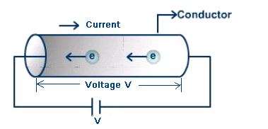
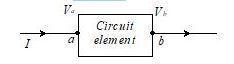
The simplest electric circuit consists of a source of e.m.f. (such as cell or battery) and
a device, which may be a resistor, capacitor, inductor or a combination of these. The
source of e.m.f. supplies electrical energy to the circuit, which is consumed or
transformed into other forms by resistor, inductor and capacitor.
In this chapter we will study direct current (d.c.) circuits, in which the direction of the
current does not change with time. In d.c. circuits with resistors only, the magnitude of
current does not change with time whereas in d.c. circuits containing capacitors and
inductors, the magnitude of current may change with time.
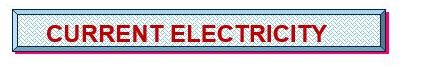
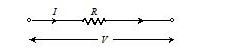
The symbols of circuit elements are as follows.

Electric current is the rate of flow of electric charges. Electric current is the result of motion of electrons or ions or holes under the influence of emf.
Charges in motion make an electric current.
Time rate of flow of charge through a cross-section is called electric current.
Suppose, a charge \(\Delta \)q passes through a given cross section Area in a short time t, then the electric current is
I = \(\frac{\Delta q}{\Delta t}\)
More precisely, the instantaneous current at a given time t is
I = \(\underset{\Delta \,t\to 0}{\mathop{\lim }}\,\frac{\Delta q}{\Delta t}=\frac{dq}{dt}\)
If the current is steady (i.e., it does not change with time), then the charge q flowing through is just proportional to time t, and we have
I =\(\frac{q}{t}\)
 (for steady current)
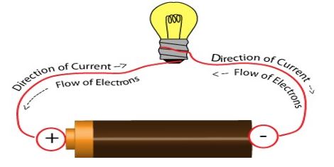
- Conventionally, the direction of current is taken to be the direction of flow of positive charge, (i.e., the direction of the field).
- In a conductor (such as copper, aluminum, etc.) the current flows due to the motion of free electrons (negatively charged particles). Hence, the direction of electric current is opposite to the direction of flow of electrons.
- In semiconductors, the current is carried by both the electrons (negative) and holes (positive). Hence, we say that in semiconductors there are two types of charge-carriers, viz., electrons and holes. In a discharge tube, the charge carriers are positive ions and negative electrons. In an electrolyte, the current flows due to the motion of both the positive ions and negative ions.
- In case of semiconductors, electrolytes and discharge tubes, though the positive and the negative charge move in opposite directions, the current due to them will be in the same direction.
- Furthermore, though the positive and negative charges are equal, their contributions to current are usually not the same. The heavier charge-carriers move slower and their contribution to electric current is less than that of lighter ones.
Current is a scalar because it does not obey the laws of vector addition:
Ø the device which converts chemical energy into electrical energy is called as ‘CELL’.
Ø Cell is a source of EMF. It converts chemical energy into electrical energy.
Ø When connected between the ends of a conductor, a cell maintains constant potential difference between the ends of the conductor.
Ø Current through the following conductor does not change with change in cross- sectional area. i.e. il = i2 =i3.
Current due to translator motion of charge:
If n particles each having a charge q pass across a given area in time t then
\(i=\frac{nq}{t}\)
If there are n particles per unit volume each having a charge q and moving with velocity v, the current through cross-section A is i=nqvA.
Current Due to Rotatory Motion of Charge :
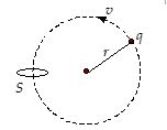
If a point charge q is moving in a circle of radius r with speed v,then its time period T = (2r/v).So, through a given cross-section (perpendicular to motion), the current is
\(I=\frac{q}{t}=\frac{q}{T}=\frac{qv}{2\pi r}\)
Current Carriers:
Ø The charged particles whose flow is in a definite direction constitutes the electric current and are called current carriers. In different situations current carriers are different.
Ø Solids: In solid conductors like metals, current carriers are free electrons.
Ø Liquids: In liquids, current carriers are positive and negative ions.
Ø Gases: In gases, current carriers are positive ions and free electrons.
Ø Semiconductors: In semiconductors, current carriers are holes and free electrons.

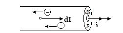
Electric current may be distributed non-uniformly over the surface through which it passes. Hence, in order to characterize the current in greater detail, we introduce the concept of current density vector \(\vec{J}\) at a point, defined as follows :
(1) The magnitude of \(\vec{J}\) is equal to the current per unit area surrounding that point and normal to the direction of charge flow. Thus,
J = \(\frac{dI}{dS}\)
(2) The direction of \(\vec{J}\) is the same as the direction of velocity vector \({\vec{v}}\) of the ordered motion of positive charge-carriers.
If the current is due to the motion of both positive and negative charges, the current density is given by
\(\vec{J}\)= \({{\rho }_{+}}{{\vec{u}}_{+}}+{{\rho }_{-}}{{\vec{u}}_{-}}\)wherer+and r-are volume densities of positive and negative charge carriers, respectively, and \({{\vec{u}}_{+}}\) and \({{\vec{u}}_{-}}\) are their velocities.
In conductors, the charge is carried only by electrons. Therefore,
 \(\vec{J}\)=\(={{\rho }_{-}}{{\vec{u}}_{-}}\)
Here, the value of r is negative. Hence the directions of \(\vec{J}\) and \({{\vec{u}}_{-}}\) are opposite to each other.
If at point P current DI passes normally through area Ds as shown. Current density \(\vec{J}\) at P is given by
\(\vec{J}=\underset{\Delta s\to 0}{\mathop{lim}}\,\frac{\Delta I}{\Delta S}\vec{n}\) or \(\vec{J}=\frac{dI}{ds}\vec{n}\)
In general, if the cross-sectional area is not normal to the current, the cross-sectional area normal to current will be ds cosq and so in this situation
\(J=\frac{dI}{dS\cos \theta }\)
dI = J dS cos q
or dI = \(\vec{J}.d\vec{S}\)
or I = \(\int{\vec{J}.d\vec{S}}\)
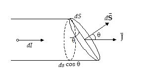
Thus, the electric current is the flux of current density.
Note the following important points about current density.
(1) Both current I and current density \(\vec{J}\)have directions, by definition current density \(\vec{J}\) is a vector while current I is a scalar.
(2) Though the charge density rc is defined as charge per unit volume, it may have different values at different points, as
rc = \(\underset{\Delta V\to 0}{\mathop{\lim }}\,\frac{\Delta q}{\Delta V}\)
(3) For uniform flow of charge through a cross-section normal to it, we have
I = nqvS
\(\vec{J}\)= \(\frac{I}{S}\vec{n}=\left( nqv \right)\vec{n}\) (as nv = rc) or
\(\vec{J}\)=nq \({\vec{v}}\) = \({{\rho }_{c}}\vec{v}\)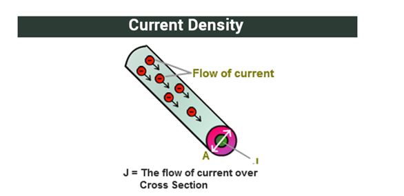
- If the current density is constant, I µ S. Thus, for a given current density, lesser the area of cross-section, the lesser will be the current. [Fig. (B)].
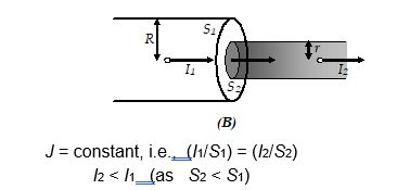
- If the cross-section is constant, I µ J. Thus, for a given cross-sectional area, the greater the current density, the greater will be the current.

1.A steady current is set up in a metallic wire of non-uniform cross-section. Then the drift velocity related the area of cross-section (A) as
Solution: \({{V}_{d}}\propto {{A}^{-1}}\)
2.A steady current passes through a wire of non-uniform cross-section. The quantities dependent on the cross-section are
Solution: The quantities dependent on the cross-section are drift velocity.

1.In a hydrogen atom, an electron is revolving with an angular frequency 6.28 rad/s around the nucleus. Then the equivalent electric current is .....\(\times {{10}^{-19}}\) A
Solution: \(i=\frac{\omega q}{2\pi }\)\(=\frac{6.28\times 1.6\times {{10}^{-19}}}{2\times 3.1}\) = 1.6
2.The current passing through a conductor is 5 amperes. The charge that passes through that conductor in 5 minutes is
Solution:\(i=\frac{q}{t}\) =1500.

1.The current in a wire varies with time according to the relation
i = a + bt2,
where current i is in ampere and time t is in second; a = 4A, b = 2As-1.
(a) How many coulombs pass a cross-section of the wire in the time interval between t = 5 s and
t = 10 s?
(b) What constant current could transport the same charge in same time interval?
Solution:
(a) q = \(\int\limits_{5}^{10}{i\,\,dt}=\int\limits_{5}^{10}{\left( 4+2{{t}^{2}} \right)\,\,dt}\)
= \(\left| 4t+\frac{2}{3}{{t}^{3}} \right|_{5}^{10}=4\left( 10-5 \right)+\frac{2}{3}\left( 1000-125 \right)\) = 603.33 C
(b) Ie = \(\frac{\Delta q}{\Delta t}=\frac{603.33}{10-5}\) = 120.67 A .
2.In the Bohr model of hydrogen atom, the electron is pictured to rotate in a circular orbit of radius 5´10-11 m, at a speed of 2.2´106 m/s. What is the current associated with electron motion?
Solution:
The time taken to complete one rotation is
T = \(\frac{2\pi r}{v}\)
Therefore, the current is
I = \(\frac{q}{t}=\frac{e}{T}=\frac{ev}{2\pi r}=\frac{1.6\times {{10}^{-19}}\times 2.2\times {{10}^{6}}}{2\times 3.14\times 5\times {{10}^{-11}}}\)=1.12 MA

1.One end of the aluminium wire whose diameter is 2.5 mm is welded to one end of a copper wire whose diameter is 1.8mm. The composite wire carries a current I of 1.3A. What is the current density in each wire?
Solution:
The current density is given by \(j=\frac{I}{S}\)
For Aluminium wire, \({{S}_{AI}}=\frac{\pi {{d}^{2}}}{4}=\frac{\pi }{4}{{(2.5\times {{10}^{-3}})}^{2}}\)
\(=4.91\times {{10}^{-6}}{{m}^{2}}\)
\({{j}_{AI}}=\frac{I}{{{S}_{AI}}}=\frac{1.3}{4.91\times {{10}^{-6}}}\)
\(=2.6\times {{10}^{5}}\text{A}{{\text{m}}^{-2}}=26A\,\text{c}{{\text{m}}^{-2}}\)
For copper wire, \({{S}_{\text{Cu}}}=\frac{\pi {{d}^{2}}}{4}=\frac{\pi }{4}{{(1.8\times {{10}^{-3}})}^{2}}\)
\(=2.54\times {{10}^{-6}}{{\text{m}}^{2}}\)
\({{j}_{\text{Cu}}}=\frac{I}{{{S}_{\text{Cu}}}}=\frac{1.3}{2.54\times {{10}^{-6}}}\)
\(=5.1\times {{10}^{5}}\text{A}{{\text{m}}^{-2}}=51A\,\,\text{c}{{\text{m}}^{-2}}\).
2.In the above illustration, if the resistivity of aluminum and copper is 2.75 × 10⁸Wand 1.69 × 10⁻⁸Wm, respectively, then determine the magnitude of electric field in each wire?
Solution:
Using differential form of Ohm’s law
\(j=\frac{E}{\rho }\)
We have \({{E}_{\text{Al}}}={{\rho }_{\text{Al}}}\,\,{{j}_{\text{Al}}}=(2.75\times {{10}^{-8}})\,\,(2.6\times {{10}^{5}})\)
\(=7.15\times {{10}^{-3}}\text{V}{{\text{m}}^{-1}}\)
and \({{E}_{\text{Cu}}}={{\rho }_{\text{Cu}}}\,\,{{j}_{\text{Cu}}}=(1.69\times {{10}^{-8}})\,\,(5.1\times {{10}^{5}})\)
\(=8.62\times {{10}^{-3}}\text{V}{{\text{m}}^{-1}}\)
-
CURRENT ELECTRICITY
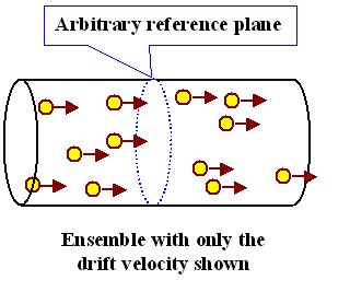
The drift velocity is the average uniform velocity acquired by free electrons inside a metal by the application of an electric field which is responsible for current through it.
Free electrons, under the influence of thermal agitation, move randomly throughout the metallic conductor from one point to another in an irregular manner in all possible directions as shown in Fig. (A). However, if a source of potential difference is applied across the two ends of the conductor, the electrons gain velocities tending them to move from negative to positive side of the conductor. Average value of these
velocities is termed as drift velocity. The drift velocity of the electrons is no doubt superimposed on their random velocity, but in fact this is the cause for net transportation of the charge along the conductor and hence results in a current flow.
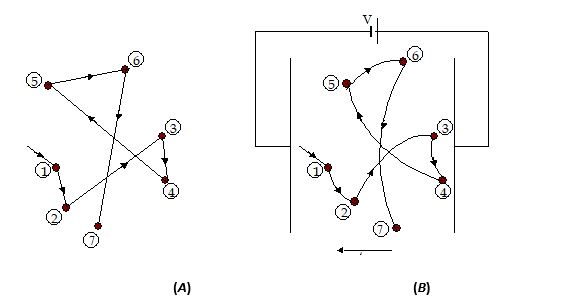
In absence of any electric field [Fig.(A)], the random motion of electrons does not contribute to any current. The number of electrons crossing any plane from left to right is equal to the number of electrons crossing from right to left (otherwise metal will not remain equipotential).
When an electric field is applied, due to electric force the path of electrons in general becomes curved instead of straight lines and electrons drift opposite to the field [Fig.(B)].
The velocity with which an electron gets drifted in a metallic conductor under the application of an external electric field is called drift velocity.
Ø The average velocity of electron in a direction opposite to field when an electric field is applied to the metallic conductor is also called drift velocity. Over number of collisions, drift velocity can be uniform.
- \({{V}_{d}}\) is in the order of \({{10}^{-4}}m{{s}^{-1}}\).
Let n be the no. of free electrons per unit volume under the application of electric field to the
conductor of cross section A. If \({{V}_{d}}\) be the drift velocity then
Current =\(i=\frac{Ne}{t}\) , where=\(n=\frac{N}{vol}\),
\(i=nA\left( \frac{l}{t} \right)e\) , N = n (volume) = \(n\left( Al \right)\)
\(i=nA{{V}_{d}}e\) N: Total free electrons
\({{V}_{d}}=\frac{i}{nAe}\) e: Charge of electron.
\({{\text{v}}_{d}}=\frac{\text{i}}{neA}=\frac{J}{ne}=\frac{\sigma E}{ne}=\frac{E}{\rho ne}=\frac{V}{\rho lne}\)
\(where\,\sigma =\frac{\text{1}}{\rho }\), \({{V}_{d}}=\frac{l}{t}\) .
Current in a Conductor:
Consider a conductor of uniform cross-sectional area S. If n is the number of free electrons per unit volume, the charge per unit volume is ne. If vd is the drift velocity, electrons move a distance vd in one second. Therefore, the volume moved in one second is vdS. Thus, the current,
I = \(\frac{ch\arg edensity\times volume}{time}=\frac{\left( ne \right)\times \left( {{v}_{d}}s \right)}{1}=ne{{v}_{d}}s\)
J = \(\frac{I}{S}=ne{{v}_{d}}\) or vd = \(\frac{J}{ne}\).
Metals (conductors) have large number of free electrons per unit volume (» 1028/m3). Therefore, the drift velocity is very small (»10-4 m/s) compared to random speed of electrons at room temperature (» 106 m/s).
The area of cross-section, length and density of a piece of a metal of atomic mass 60 gm/mole are 10-6 m2, 1 m and 5´103 kg/m3 respectively. Find the number of free electrons per unit volume if every atom contributes one free electron. Also find the drift velocity of electrons in the metal when a current of 16 A passes through it. Given that Avogadro’s number NA = 6´1023/mole and charge on an electron e = 1.6´10-19 C.
According to Avogadro’s hypothesis,
\(\frac{N}{{{N}_{A}}}=\frac{m}{M}\) so n = \(\frac{N}{V}={{N}_{A}}\frac{m}{VM}=\frac{{{N}_{A}}d}{M}\) (as d = \(\frac{m}{V}\))
n = \(\frac{6\times {{10}^{23}}\times \left( 5\times {{10}^{3}} \right)}{\left( 60\times {{10}^{-3}} \right)}\) = 5´1028 /m3
Now as each atom contributes one electron, the number of electrons per unit volume is also the same.
J = \(\frac{I}{S}=\frac{16}{{{10}^{-6}}}\)= 16´106 A/m2.
vd = \(\frac{J}{ne}=\frac{16\times {{10}^{6}}}{\left( 5\times {{10}^{28}} \right)\times \left( 1.6\times {{10}^{-19}} \right)}=\) 2 ´ 10-3 m/s .
diagram:
Relaxation Time(t):
The average time between two successive collisions suffered by electrons inside given conductor when electric field is applied is called relaxation time It is in the order of \({{10}^{-14}}\)s.
Relation between Relaxation time and drift velocity:
When electron starts from rest ,if it acquires drift velocity \({{V}_{d}}\) with an acceleration ‘a’ in
the presence of electric field E then
(It is average motion between two successive collisions)
\({{V}_{d}}=at\)
\({{V}_{d}}=\frac{Ee}{m}t\)...........(1)
\({{\bar{V}}_{d}}=\frac{-e\bar{E}}{m}t\)
But \({{V}_{d}}=\frac{i}{neA}\) ..........(2)
from (1) & (2) current \(i=\frac{nE{{e}^{2}}At}{m}\)
\(\frac{V}{R}=\frac{nE{{e}^{2}}At}{m}\) .But potential\(V=El\)

\(\frac{El}{R}=\frac{nE{{e}^{2}}At}{m}\)
Resistance=\((R)=\frac{m}{n{{e}^{2}}t}\frac{\ell }{A}\) ,
Resistivity=\(\rho =\frac{m}{n{{e}^{2}}t}\) .
Mobility (m):
In a substance, although the amount of charge on a positive charge-carrier and on a negative charge–carrier may be the same, but the two types of carriers may not give equal contribution to electric current. For example, in a semiconductor, (such as Ge or Si), the two types of charge-carriers are electrons (negative) and holes (positive). When an electric field is applied, the electrons are found to drift more than the holes. We say that the mobility of electrons is more than that of holes.
Mobility (m) of a charged particle in a substance is defined as the drift velocity per unit field applied,
m = \(\frac{{{v}_{d}}}{E}\)
The units of mobility are ‘m/s per V/m’ or m2/Vs.
For a conductor we can write
J = nevd = mneE
An intrinsic semiconductor has same number of holes and electrons, and the amount of charge on them is also same. Hence
J = Current density due to drift of electrons + Current density due to drift of holes
= Je+ Jp = enmnE + epmpE
\ J = en (mn + mp)E (as n = p).

1.A current of 200mA flows in a silver wire of radius 0.8mm.
(a) Find the drift speed of the electrons.
(b) The electric field within the wire.
The free electrons density is 5.8 × 1028m–3. The resistivity of silver is 1.62 × 10⁻⁸Wm.
Solution: (a) 1.07 × 10⁻⁵ ms–1
(b) 1.49 × 10⁻³
2.The drift speed of an electron in a metal is of the order of?
Solution:
The drift speed of an electron in a metal is of the order of 10–4 m/s

1.A current flows in a wire of circular cross section with the free electrons travelling with drift velocity. If an equal current flow in a wire of twice the radius, new drift velocity is
Solution:
\({{V}_{d}}\propto \frac{1}{{{r}^{2}}}\) =\(\frac{\overrightarrow{V}}{4}\)
2.A copper wire of cross-sectional area 2.0 \(m{{m}^{2}}\) , resistivity = \(1.7\times {{10}^{-8}}\,\,\Omega m\) , carries a current of 1 A. The electric field in the copper wire is
Solution:
\(E=\frac{i\rho }{A}\) =\(8.5\times {{10}^{-3}}\,V/m\) .

1.A wire of diameter 0.02 meter contains 1028 free electrons per cubic meter. For an electric current of 100 amperes, the drift velocity for free electrons in the wire is most nearly?
Solution:
Drift velocity is the average velocity of a carrier that is moving under the influence of an electric field
Velocity: v = L/t
In a wire with length L and cross-sectional area A, there are n electrons with charge qe per cubic meter.
Total number of mobile electrons in the wire, Q = nqeLA
Current: I = Q/t = nqeLA/t = nqevA
v = I/nqeAqe = charge of an electron = 1.6 × 10⁻¹⁹ C
n = 1028 electrons/m³
A = πr² = 0.5π × 10−4
I =100 Ampere.
v = 102 / (1028× 1.6 × 10−19× 0.5π × 10−4)
= 102−28+19+4 / (1.6 × 0.5π)
≈ 10−4.
.
-
CURRENT ELECTRICITY
It is the device mainly used to measure emf of a given cell and to compare emf’s of cells. It is also used to measure internal resistance of a given cell.
P.D across the balancing length of potentiometer wire is equal to emf of the cell in the secondary circuit.
Potentiometer is also known as ideal voltmeter, because it measure the emf of the cell without drawing current from cell. So potentiometer is preferred than voltmeter to measure the emf of the cell.
Uses of Potentiometer :
Potentiometer is used
i) to measure the unknown emf of the cell
ii) to compare the emf’s of two cells
iii) to determine the internal resistance of the cell (r)
iv) to measure the current in the circuit
v) to measure the P.D between two points
vi) to measure thermo emf
vii) to calibrate ammeter
viii) to calibrate voltmeter.
Circuit Diagram:
Potentiometer consists of a long resistive wire AB of length L (about 6m to 10m long) made up of mangnine or constantan and a battery of known voltage ‘e’ and internal resistance ‘r’ called supplier battery or driver cell. Connection of these two forms primary circuit.
One terminal of another cell (whose emf E is to be measured) is connected at one end of the main circuit and the other terminal at any point on the resistive wire through a galvanometer G. this forms the secondary ciruit. Other details are as follows
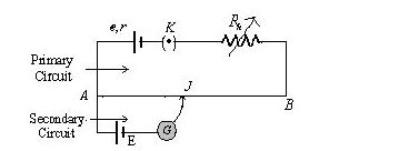
J = jockey
K = key
R = resistance of potentiometer wire
\(\rho \) = Specific resistance of potentiometer wire
Rh = Variable resistance which controls the current through the wire AB.
The specific resistance (\(\rho \)) of potentiometer wire must be high but its temperature coefficient of resistance (\(\alpha \)) must be low.
All higher potential points (terminals) of primary and secondary circuits must be connected together at point A and all lower potential points must be connected to point B or jockey.The value of known potential difference a cross the balancing length must be greater than the value of unknown potential difference to be measured.
The potential gradient must remain constant. For this the current in the primary circuit must remain constant ant the jockey must not be slided in contact with wire.
The diameter of potentiometer wire must be uniform everywhere.
Comparing Two Cells using Potentiometer
A potentiometer is commonly used for comparison of emfs of cells. A battery X is connected across a long uniform wire AB. The cells E1 and E2 (whose emfs are to be compared) are connected as shown along with a galvanometer.
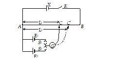
First the key S1 is pressed which brings E1 in the circuit. The sliding contact C is moved till the galvanometer shows no deflection. Let the length AC = L1. Next S1 is opened and S2 is closed. This brings E2 in the circuit. Let C¢ be the new null point and let AC¢ = L2. Then, clearly, \(\frac{{{E}_{1}}}{{{E}_{2}}}=\frac{{{L}_{1}}}{{{L}_{2}}}\)
Potential Gradient (x):
Potential difference (or fall in potential) per unit length of wire is called potential gradient
i.e. \(x=\frac{v}{l}\frac{volt}{m}\)
where V = iR = \(\left( \frac{e}{R+{{R}_{h}}+r} \right)\frac{R}{L}\)
\(x=\frac{v}{l}=\frac{iR}{L}=\frac{i\rho }{A}=\frac{e}{\left( R+{{R}_{h}}+r \right)}\frac{R}{L}\)
Potential gradient directly depends upon.
a) The resistance per unit length\(\frac{R}{L}\) of potentiometer wire.
b) The radius of potentiometer wire (i.e. Area of cross-section)
c) The specific resistance of thematerial of potentiometer wire (i.e\(\rho \))
d) the current flowing through potentiometer wire
Ø Potential gradiaent indirectly depends upon
a) The emf of bettery in the primary circuit (i.e.E)
b) The resistance of rheostat in the primary circuit (ie\({{R}_{h}}\).)
Working: suppose jockey is made to touch a point J on wire then potential difference between A and J will be \(V=xI\)
At this length (l) two potential differences are obtained
i) V due to battery ‘e’ and
(ii) E due to unknown cell.
It \(V>E\)then current will flow in galvanometer circuit in one direction
If \(V<E\)then current will flow in galvanometer circuit in opposite direction
If \(V=E\)then no current will flow in galvanometer circuit. This condition to known as null deflection position, length l is known as balancing length.
In balanced condition\(E=xl\)
\(E=xl=\frac{V}{L}l=\frac{iR}{L}l=\left[ \frac{e}{R+{{R}_{h}}+r} \right].\frac{R}{L}\times l\)
If V, x and E are constant then
\(L\propto l\Rightarrow \frac{{{x}_{1}}}{{{x}_{2}}}=\frac{{{L}_{2}}}{{{L}_{1}}}=\frac{{{l}_{2}}}{{{l}_{1}}}\)
Sensitivity of potentiometer
A potentiometer is said to be more sensitive, if it measures a small potential difference more accurately.
ØThe sensitivity of potentiometer is assessed by its potential gradient. The sensitivity is inversely proportional to the potential gradient.
ØIn order to increase the sensitivity of potentiometer
ØThe resistance in primary circuit will have to be increased.
ØThe length of potentiometer wire will have to be increased so that the balanceing length may be measured more accurately.
Ø The sensitivity is independent of resistance of potentiometer wire in the absence of primary circuit resistance.
Difference between voltmeter and potentiometer:
Voltmeter Potentiometer
1.It’s resistance is high 1. Its resistance is
but finite. It draws infinite. It does not
some current from draw any current
source of emf from the source of
unknown emf
2. The potential difference 2.The potential measured by it is difference
lesser than the actual measured by it is
potential difference. Its equal to actual
sensitivity is low. potential difference.
Its sensitivity is high.
3. It is a versatile 3. It measures only
instrument emf or potential
difference.
4. It is based on 4. It is based on zero
deflection method deflection method.
- Potentiometer is also known as ideal voltmeter, because it measure the emf of the cell without drawing current from cell. So potentiometer is preferred than voltmeter to measure the emf of the cell.
- If jockey is pressed to the left of balancing point, current flows from secondary to primary circuit
- If jockey is pressed to the right of balance point, current flows from primary to secondary circuit.
- If jockey is pressed at balance point, current flow between primary and secondary is zero.
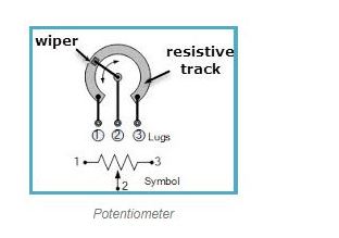
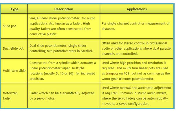
Types of Potentiometers:
A potentiometer is also commonly known as pot. These potentiometers have three terminal connections. One terminal connected to a sliding contact called wiper and the other two terminals are connected to a fixed resistance track. The wiper can be moved along the resistive track either by use of a linear sliding control or a rotary “wiper” contact. Both rotary and linear controls have the same basic operation.
The most common form of the potentiometer is the single turn rotary potentiometer. This type of potentiometer is often used in audio volume control (logarithmic taper) as well as many other applications. Different materials are used to construct potentiometers, including carbon composition, cermet, conductive plastic, and the metal film.
Rotary Potentiometers
These are the most common type of potentiometers, where the wiper moves along a circular path.
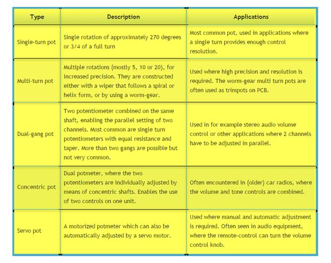
Linear Potentiometers
In these types of Potentiometers the wiper moves along a linear path. Also known as slide pot, slider, or fader.
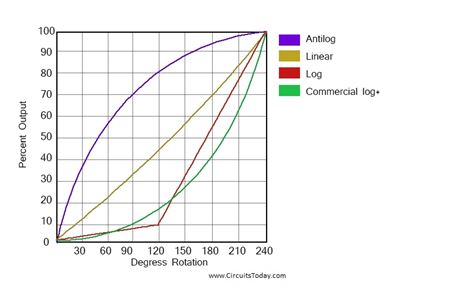
Characteristics of Potentiometers
Some of the characteristics of a potentiometer are:
TAPER: The law of pots or the taper of pots is one such characteristic of potentiometer in which one needs a prior knowledge, to pick the right device for the desired application. It is nothing but a ratio between the wiper position and the resistance. This ratio when plotted may be linear, logarithmic or antilogarithmic, as shown in figure.
MARKING CODES: While selecting a potentiometer, you need to know the maximum value of resistance it can attain. For this purpose, the manufactures use marking codes, which indicate the same. For example, a pot with a resistance of 100K marked on it means, the maximum limit of the pot is 100kΩ.
Since, we also need to know the taper of the pot, the manufacturers use marking codes for indicating the taper of the pot as well. The marking codes differ from a region to region. One must have prior knowledge of what a code stands for.
RESOLUTION: As we vary the resistance in the pot, there is a minimum amount of resistance that can be changed. This is known as the resolution of the pot. For example, if I say the resistance of pot is 20kΩ, with a resolution of 0.5, the minimum change in resistance will be 0.5Ω, and the values that we get for the smallest change will be 0.5,1.5,2Ω and so on.
HOP ON HOP OFF RESISTANCE: Like we have seen in the construction part of this article that the resistive element is connected in between the two terminals. These terminals are made of very low resistance metal. Hence, whenever the wiper enters or exits this region, there will be a sudden change in the resistance. This characteristic of the pot is called, hop on hop off resistance.
-
CURRENT ELECTRICITY

Consider the following statements :
A: As no current is drawn from the cell in the secondary of a potentiometer at the time of obtaiang the balance point , its emf can be accurately measured.
B: The sensitivity of a potentimeter depends on the potential gradient along the wire , the more the potential gradient the less the sensitivity
1) A and B are false 2) A is true , B is false
3) A and B are true 4) A is false, B is true
Solution:
A and B are true
2.A potentiometer is superior to voltmeter for measuring a potential because
1) voltmeter has high resistance
2) resistance of potentiometer wire is quite low
3) potentiometer does not draw any current from the unknown source of emf. to be measured
4) sensitivity of potentiometer is higher than that of a voltmeter.
Solution:
potentiometer does not draw any current from the unknown source of emf. to be measured.

Q1. The resistivity of a potentiometer wire is given as 5 * 10-6 Ωm. The area of cross section of the wire is given as 6 * 10-4 m2. Find the potential gradient if a current of 1 A is flowing through the wire.
Solution:
K = V/L
= IR/L
= (IρL/A)/L
= Iρ/A
Substituting the values we get K =1* 5 * 10-6/6 * 10-4 m2 = 0.83 * 10-2 v/m.
2. A potentiometer of length 1 m has a resistance of 20 Ω. It is then connected with a battery of 8 V and resistor of 5 Ω in series with the wire. Calculate the emf of the primary cell when it gives a balance point at 60 cm.
Solution:
The length of the wire L = 100 cm
Resistance, R = 20 Ω
Rs = 5 Ω
E = 8 V, L1 = 60 cm
Current I = 8/20 + 5 = 8/25 = 0.32 A
Potential difference across the wire V = IR = 0.32 * 20 = 6.4 V.
Thus according to the principle of potentiometer, E2 /V = L1 /L
E2 = (V/L) * L1 = (6.4/100) * 60
= 3.84 V..

2. A potentiometer has a wire of length 8 m and the resistance of the wire is 20 Ω. It is connected in series with a cell of emf 2 V and an internal resistance 2 Ω and a rheostat. Find the value of the resistance in rheostat when the potential drop along the wire is 20 µv/mm.
Solution:
The given values are
L = 8 m, R = 20 Ω, E = 2 V, r = 2 Ω
The potential drop per length mentioned here is the potential gradient.
So K = 20 µv/mm.
We know that K = V/L
= IR/L
= ER/(R + r + Rh)L
So 20 * 10-6/10-3 v/m = 2 * 20/(20 + 2 + Rh) 8
= 20 * 10-3 = 40/(22 + Rh) 8
20 * 10-3 = 5/22+ Rh
22 + Rh = 5 * 103/20 = 250
Rh = 250 – 22
= 228 Ω.
2.A battery of emf 4 V is connected across a 10 m long potentiometer wire having a resistance per unit length 1.6 W m–1. A cell of emf 2.4 V is connected so that its negative terminal is connected to the low potential end of the potentiometer wire and the other end is connected through a galvanometer to a sliding contact along the wire. It is found that the no-deflection point occurs against the balancing length of 8 m. Calculate the internal resistance of the 4 V battery.
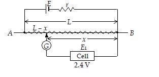
Solution:
emf of cell =(potential gradient) ´ (balancing length)
\({{E}_{1}}=\frac{{{V}_{AB}}}{L}\times x\)
or \(2.4=\frac{{{V}_{AB}}}{10}\times 8\) Þ VAB = 3 V
Consider the loop containing E. Applying potential divider concept,
\({{V}_{AB}}=E\frac{{{R}_{AB}}}{{{R}_{AB}}+r}\)
Þ \(3=4\frac{1.6\times 10}{1.6\times 10+r}\)
Þ r = 16/3 W.
Note that as there is no current through the cell and galvanometer, the battery E, the internal resistance r and the potentiometer wire AB are in series.

1.A potentiometer made from homogenous resistance wire of length l and resistance Rl = al is used to changed voltage at an appliance of resistance R. Find the voltage across and current through a resistor R as a function of the distance x of the sliding contact from the end of the potentiometer.
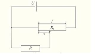
Solution:
The voltage across and current through the resistor R as functions of the distance x of the sliding contact from the end of the potentiometer are given by the expressions:

The Wheatstone network is used to determine unknown resistances. The metre bridge is an instrument based on the balancing condition of the Wheatstone network. The resistances R1 and R2 are two parts of a long wire PQ (usually 1 m long) (R1 = kL1, R2 = kL2) The portion PA of the wire offers resistance R1 and the portion QA offers resistance R2. The sliding contact at A is adjusted so that the galvanometer reads zero. In the no-deflection condition,
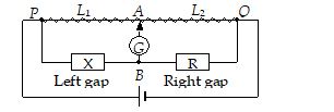
\(\frac{{{R}_{1}}}{{{R}_{2}}}=\frac{X}{R}\text{ }\Rightarrow \text{ }X=R\left( \frac{{{R}_{1}}}{{{R}_{2}}} \right)\)
or \(X=R\frac{{{L}_{1}}}{{{L}_{2}}}\)
If R is a known resistance, then X can be measured by measuring the lengths L1 and L2.
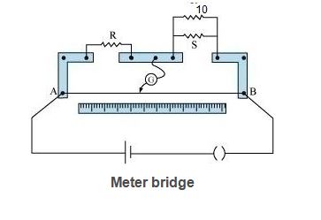
Meter bridge is also known as the Slide Wire Bridge. It consists of a wire whose length is one meter and has uniform cross sectional area. Now the wire is stretched along a meter scale. The bridge has two metallic strips which is in reverted L shape on either side of the wire. These metallic strips act as holders for the wire. The wire is being clamped to the strips.These two metallic strips are made up of metals like copper. The bridge consists of another metallic strip which is placed between those two strips with a gap between them. So totally there are five leads on the bridge.
A resistance box R and an unknown resistance S is connected across the two gaps of the metallic strips as shown in the figure. One end of the galvanometer is connected to the middle lead of the metallic strip which is placed between the L shaped strips. The other end of the galvanometer is connected to a jockey. The jockey is used to slide on the bridge wire. It is a metal rod with one end as knife edge.
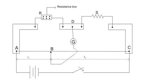
Now adjust the value of resistance in the resistance box and slide the jockey along the wire. This process is to be done until the galvanometer shows a zero or null deflection. Consider at point B the galvanometer showed zero deflection. So now the jockey is connected to the point B on the wire. Thus the distance from the point A to B is taken as L1 cm. Then the distance from point B to point C is L2 cm that is 100 - L1 cm. Now the meter bridge becomes similar to the Wheatstone bridge. The meter bridge now is drawn as Wheatstone bridge for more clearance.
Meter bridge to Wheatstone bridge
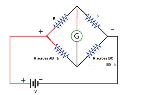
We know that R = ρ L /A, where R is the resistance, ρ is the resistivity, L is the length of the wire and A is the area of cross section of the wire. So the resistance across the portion AB of the wire is Rw L1 and that the resistance across the point BC is Rw (100 - L1). Rw is the resistance of the whole wire. That is according to Wheatstone bridge we get
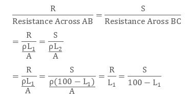
This is the equation
So to find the unknown resistance S we have S = R (100 - L1) / L1.
Draw backs with Metre Bridge :
i) Due to the contact resistance at the terminals to which wire is in contact, There will be an error in the measurement. Hence we cannot measure low resistance.
ii) Metre bridge wire may not be of exactly one metre length because of draging of jockey on the wire this gives rise to an error in the reading.
iii) Bridge will be more sensitive when = 1 i.e ; l1 is 50 cm. Hence with a given standard resistance ‘S’ we cannot accurately determine very high resistance.
iv) With a meter bridge it is advised to obtain a balancing length ‘l’ in the middle one third of the wire for more accuracy.

1.In metrebridge experiment, the known and unknown resistances in the two gaps are interchanged.The error so removed is
Solution: The error so removed is end correction
2. In a metrebridge, metal wire is connected in the left gap, standard resistance is connected in the right gap and balance point is found. If the metal wire in the left gap is heated, the balance point
Solution:
If the metal wire in the left gap is heated, the balance point shifts towards right.

1. When an unknown resistance and a resistance of 4 are connected in the left and right gaps of a Meter bridge, the balance point is obtained at 50cm. The shift in the balance point if a 4 resistance is now connected in parallel to the resistance in the right gap is
Solution:
\(\frac{x}{y}=\frac{50}{50}\) --- (1)
\(\frac{4}{2}=\frac{l}{\left( 100-l \right)}\)----- (2)
\(\frac{4}{2}=\frac{l}{\left( 100-l \right)}\)
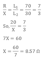
2.In a meter bridge, the gaps are closed by resistances 2 and 3 ohms. The value of shunt to be added to 3 ohm resistor to shift the balancing point by 22.5 cm is
Solution:
\(\frac{2}{3}=\frac{l}{100-l}\)\(\Rightarrow l=40\text{ }cm\)
\(\frac{2}{\frac{3r}{3+r}}=\frac{62.5}{100-62.5}\)= 2


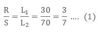
1. In a meter bridge, there are two unknown resistance R1 and R2. Find the ratio of R1 and R2 if the galvanometer shows a null deflection at 30 cm from one end?
Solution:
The null deflection in the galvanometer is given as 30 cm from one end.
So consider L1 = 30 cm
So L2 = 100 – 30 = 70 cm
Thus the ratio of the unknown resistance can be found as
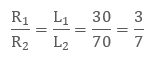
Thus R1: R2 = 3: 7
2. A 20 Ω resistor is connected in the left gap and an unknown resistance is connected in the right gap of the meter bridge. Also the null deflection point is shifted by 40 cm when the resistors are interchanged. Find the value of unknown resistance?
Solution:
In the first case the deflection point is taken as L1. Let the balance point gets shifted to L2 by 40 cm when the resistors are interchanged.
So we get L1 - L2 = 40
Also we know L1 + L2 = 100
Solving these two equations we get L2 = 30 cm and L1 = 70 cm.

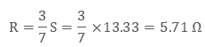
1.the meter bridge, the null deflection is shown on the galvanometer which is at a distance of 30 cm from one point. When a known resistance of 10 Ω is connected in parallel with another unknown resistance S the null deflection shows at 50 cm from the same point. Find the unknown resistance of R and S.
Solution:
In the first case L1 = 30 cm
As the resistors are connected in parallel we know that the equivalent resistance is R1 R2 / R1 + R2
= 10 * S / 10 + S
In the second case L1 = 50 cm So L2 = 100 – 50 = 50
So according to the formula
R / S = 1
= R / (10 S / 10 + S) = 1
So R = 10 S / 10 + S
Substituting the value of R in equation 1we get
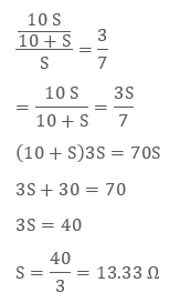
From equation 1 we get
Electrical Energy:
The electric energy consumed in a circuit is defined as the total workdone in maintaing the current in an electric circuit for a given time.
Electrical Energy = Vit = Pt = \({{i}^{2}}Rt=\frac{{{V}^{2}}t}{R}\,\,\)
S.I. unit of electric energy is joule where
1 Joule=1watt1 sec = 1 voltampere1 sec
\(1Kwh=1000Wh=3.6\times {{10}^{6}}J\).
Electrical Power:
- The rate at which work is done in maintaining the current in electric circuit. Electrical power
\(P=\frac{W}{t}=Vi={{i}^{2}}R=\frac{{{V}^{2}}}{R}\)
- Heat energy produced due to the electric current H = \(\frac{W}{J}=\frac{Pt}{J}=\frac{E\,it}{J}=\frac{{{i}^{2}}Rt}{J}=\frac{{{E}^{2}}t}{RJ}\)
- \(H=ms\Delta t\)
Where \(s=4200J\)/Kg0C
where J is mechanical equivalent of heat.
- If radiation losses are neglected, due to heating effect of current the temperature of fuse wire will increase continuously, and it melt in time ‘t’ such that
\(H=ms\,\Delta \theta ;\frac{{{I}^{2}}Rt}{J}=ms({{\theta }_{mp}}-{{\theta }_{r}})\)
\(t=\frac{{{\pi }^{2}}{{r}^{4}}s\left( {{\theta }_{mp}}-{{\theta }_{r}} \right)J}{{{I}^{2}}\rho };\,t\,\alpha \,{{r}^{4}}\)
Energy and Power in

Power delivered to a resistor is \(VI={{I}^{2}}R=\)\(\frac{{{V}^{2}}}{R}\)
\({{P}_{output}}={{V}_{ab}}I=\left( E-Ir \right)\,I=EI-{{I}^{2}}r\)
\({{P}_{input}}={{V}_{ab}}I=\left( E+Ir \right)r=EI+{{I}^{2}}r\).
Fuse Wire:
It should have high resistance and very low melting point . If i s the current passing through the fuse wire of radius r then \(\text{i}\propto {{r}^{\,\frac{3}{2}}}\)The current carrying capacity i.e. i is independant of length of the fuse wire.
Bulbs connected in Series:
- If Bulbs (or electrical appliances) are connected in series, the current through each resistance is same. Then power of the electrical appliance
\(P\propto R\,\,\,\And \,\,V\propto R\left[ \therefore P={{i}^{2}}Rt \right]\)
i.e. In series combination; the potential difference and power consumed will be more in larger resistance.
- When the appliances of power are in series, the effective power consumed (P) is i.e. In series combination; the potential difference and power consumed will be more in larger resistance.
- When the appliances of power are in series \({{P}_{1}},\,\,{{P}_{2}},\,\,{{P}_{3}}....\), the effective power consumed (P) is
\(\frac{1}{P}=\frac{1}{{{P}_{1}}}+\frac{1}{{{P}_{2}}}+\frac{1}{{{P}_{3}}}+.........\)i.e. effective power is less than the power of individual appliance.
If ‘n’ appliances, each of equal resistance ‘R’ are connected in series with a voltage source ‘V’, the power dissipated \({{\text{P}}_{\text{s}}}\)will be \({{P}_{s}}=\frac{{{V}^{2}}}{nR}\).
Bulbs connected in parallel:
- If Bulbs (or electrical appliances) are connected in parallel, the potential difference across each resistance is same. Then \(P\propto \frac{1}{R}\) and .\(I\propto \frac{1}{R}\)
i.e. The current and power consumed will be more in smaller resistance.
- When the appliances of power \({{P}_{1}},\,\,{{P}_{2}},\,\,{{P}_{3}}....\)are in parallel, the effective power consumed(P) is \(P={{P}_{1}}+{{P}_{2}}+{{P}_{3}}+.........\)
i.e. the effective power of various electrical appliance is more than the power of individual appliance.
- If ‘n’ appliances, each of resistance ‘R’ are connected in parallel with a voltage source ’V’, the power dissipated ‘Pp’ will be
\({{P}_{P}}=\frac{{{V}^{2}}}{\left( R/n \right)}=\frac{n{{V}^{2}}}{R}\)
\(\frac{{{P}_{P}}}{{{P}_{S}}}={{n}^{2}}\,\,\left( or \right)\,\,{{P}_{P}}={{n}^{2}}{{P}_{S}}\)
- This shows that power consumed by ‘n’ equal resistances in parallel is times that of power consumed in series if voltage remains same.
- In parallel grouping of bulbs across a given source of voltage, the bulb of greater wattage will give more brightness and will allow more current through it, but will have lesser resistance and same potential difference across it.
- For a given voltage V, if resistance is changed from ‘R’ to \(\left( \frac{R}{n} \right)\), power consumed changes from ‘P’ to ‘nP’\(P'=\frac{{{V}^{2}}}{R'}\) where \({R}'=\frac{R}{n}\), then
- If \({{t}_{1}},\,\,{{t}_{2}}\)are the time taken by two different coils for producing same heat with same supply, then If they are connected in series to produce same heat, time taken \(t={{t}_{1}}+{{t}_{2}}\)
If they are connected in parallel to produce same heat, time taken is .\(t=\frac{{{t}_{1}}{{t}_{2}}}{{{t}_{1}}+{{t}_{2}}}\).
Consumption of Electrical Energy:
- Unit of electrical energy consumed:
- Board of Trade Unit (B.T.U)
- B.T.U = It is the electrical consumed at the rate of 1000 joules per second in one hour
- B.T.U = 1KWH = 3.5 x 10⁶ joules
- Units of electrical energy consumed by an electrical appliance
\(\frac{\text{Number}\,\text{of}\,\text{watts}\,\text{ }\!\!\times\!\!\text{ }\,\text{Number}\,\text{of}\,\text{hours}}{\text{1000}}\)
\(\text{=Units}\text{.}\,\left( \text{KWH} \right)\)
Circuits with Capacitors:
A battery maintains a certain potential difference across its terminals. Thus, when capacitor is connected to a cell, charge flows between the capacitor and the cell until the capacitor has the same potential difference across it as that across the cell.
Capacitors in Parallel:
When a potential difference \(V\) is applied across several capacitors connected in parallel, the potential difference \(V\) is applied across each capacitor.
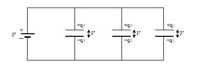
The total charge \(q\) stored on the capacitors is the sum of the charges stored on all the capacitor
Capacitors connected in parallel can be replaced with an equivalent capacitor that has the same total charge \(q\) and the same potential difference \(V\) as the actual capacitors.
Equivalent capacitance \({{C}_{eq}}\) for \(n\) capacitor in parallel is given by \({{C}_{eq}}=\sum\limits_{j=1}^{n}{{{C}_{j}}}\)
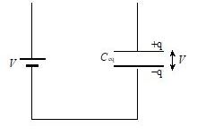
Capacitor in Series:
When a potential difference \(V\) is applied across several capacitors connected in series, the capacitors have identical charge \(q\)
 . The sum of potential differences across all the capacitors is equal to the applied potential difference \(V\)
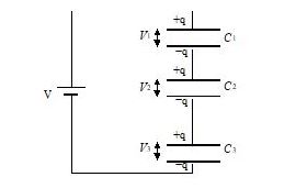
Capacitor that connected in series can be replaced with an equivalent capacitor that has the same charge \(q\)
and the same potential difference \(V\) as the actual series capacitors. Equivalent capacitance \({{C}_{eq}}\) for \(n\)capacitors in series is given by \(\frac{1}{{{C}_{eq}}}=\sum\limits_{j=1}^{n}{\frac{1}{{{C}_{j}}}}\).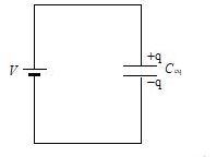

1. A resistance coil of is immersed in 42kg of water. A current of 7A is passed through it. The rise in temperature of water per minute is
Solution:
\(JQ={{i}^{2}}RtmS\Delta t={{i}^{2}}Rt\)
\(\frac{\Delta t}{t}=\frac{{{i}^{2}}R}{ms}\times 60\,\,\,\,\,\,\Delta t={{1.3}^{O}}C\)
2. A \({{5}^{0}}C\) rise in the temperature is observed in a conductor by passing some current. When the current is doubled, then rise in temperature will be equal to
Solution:
ms \(\alpha \) T \(={{i}^{2}}Rt\,\,\,\Rightarrow \Delta t\alpha {{i}^{2}}\)
\(\frac{\Delta {{t}_{1}}}{\Delta {{t}_{2}}}=\frac{i_{1}^{2}}{i_{2}^{2}}\Rightarrow \Delta {{t}_{2}}={{20}^{o}}C\)

1. Two electric bulbs marked 500 W, 220 V are put in series with 110V line. The power dissipated in each of the bulb is
Solution:\({{R}_{1}}={{R}_{2}}=\frac{{{V}^{2}}}{P}=R\)
\(i=\frac{V}{2R}\)
\( \therefore P={{i}^{2}}R=\frac{125}{4}W\)
2. An electric heater operating at 220 volts boils 5 litre of water in 5 minutes. If it is used on 110 volts, it will boil the same amount of water in
Solution:
\(H=\frac{{{V}^{2}}}{R}t\)
\(\therefore \frac{{{t}_{2}}}{{{t}_{1}}}=\frac{V_{1}^{2}}{V_{2}^{2}}=4\)= 15 minutes.
-
CURRENT ELECTRICITY

1.In the circuit shown in figure
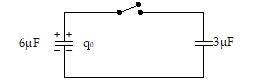
(a) Find the final charge on each capacitor after closing the switch.
(b) Also, find the percentage of energy lost.
Solution:
Since charges are distributed proportional to the capacitance, therefore
Charge on 6µF capacitor is
q6 = qo \(\left( \frac{6}{6+3} \right)\,=60\mu C\)
and on the 3µF capacitor is
q3 = qo \(\left( \frac{3}{6+3} \right)\,=\,30\mu C\)
\(\frac{\Delta {{U}_{loss}}}{{{U}_{i}}}\,=\frac{3}{3+6}=\,0.333\,\,\,\,\,(or\,\,\,33.3%)\))
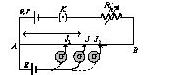
2.Consider the circuit shown in figure. What are the currents through the resistors
at
(i) t = 0,
(ii) t = ¥
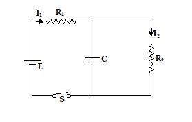
Solution:
(a) I1 = \(\frac{E}{{{R}_{1}}},\,\,\,{{I}_{2}}=0\)
(b) I1 = I2 = \(\frac{E}{{{R}_{1}}+{{R}_{2}}}\)

1.Find the current through 12Wresistor in figure.
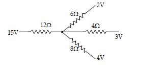
Solution:
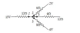
Let V be the potential at P then applying KCL at junction P.
I = \({{I}_{1}}+{{I}_{2}}+{{I}_{3}}\frac{15-V}{12}\)
= \(\frac{V-2}{6}+\frac{V-3}{4}+\frac{V-4}{8}\)
15–V= \(2(V-2)+3(V-3)+1.5(V-4)7.5V=39\)
or \(V=\frac{39}{7.5}=5.2V\)
and \(I=\frac{15-5.2}{12}=\frac{4.9}{6}A\)
2.Find the current I in figure.
(a) 1A
(b) 1.25A
(c) 2.0 A
(d) 1.75 A
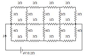
Solution:
Draw the equivalent circuit as shown in figure (a) and (b).
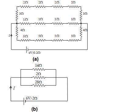
\(\frac{1}{{{R}_{eq}}}=\frac{1}{28}+\frac{1}{4}+\frac{1}{14}=\frac{1+7+2}{28}\) or Req = 2.8W
\\(I=\frac{6}{3}=2A\)
-
All topics
INTRODUCTION
In Chapter 1, all charges whether free or bound, were considered to be at rest. Charges in motion constitute an electric current. Such currents occur naturally in many situations. Lightning is one such phenomenon in which charges flow from the clouds to the earth through the atmosphere, sometimes with disastrous results. The flow of charges in lightning is not steady, but in our everyday life we see many devices where charges flow in a steady manner, like water flowing smoothly in a river. A torch and a cell-driven clock are examples of such devices. In the present chapter, we shall study some of the basic laws concerning steady electric currents.
ELECTRIC CURRENT
Imagine a small area held normal to the direction of flow of charges. Both the positive and the negative charges may flow forward and backward across the area. In a given time interval t, let q+ be the net amount (i.e.,forward minus backward) of positive charge that flows in the forward direction across the area. Similarly, let q– be the net amount of negative charge flowing across the area in the forward direction. The net amount of charge flowing across the area in the forward direction in the time interval t, then, is q = q+– q–. This is proportional to t for steady current and the quotient.
\(% MathType!MTEF!2!1!+- % feaagKart1ev2aaatCvAUfeBSjuyZL2yd9gzLbvyNv2CaerbuLwBLn % hiov2DGi1BTfMBaeXatLxBI9gBaerbd9wDYLwzYbItLDharqqtubsr % 4rNCHbGeaGqiVu0Je9sqqrpepC0xbbL8F4rqqrFfpeea0xe9Lq-Jc9 % vqaqpepm0xbba9pwe9Q8fs0-yqaqpepae9pg0FirpepeKkFr0xfr-x % fr-xb9adbaqaaeGaciGaaiaabeqaamaabaabaaGcbaGaamysaiabg2 % da9maalaaabaGaamyCaaqaaiaadshaaaaaaa!39C9! I = \frac{q}{t}\) (3.1)
is defined to be the current across the area in the forward direction. (If it turn out to be a negative number, it implies a current in the backward direction.)
Currents are not always steady and hence more generally, we define the current as follows. Let \(\Delta\)Q be the net charge flowing across a cross- section of a conductor during the time interval \(\Delta\)t [i.e., between times t and (t + \(\Delta\)t)]. Then, the current at time t across the cross-section of the conductor is defined as the value of the ratio of \(\Delta\)Q to \(\Delta\)t in the limit of \(\Delta\)t tending to zero,
\(% MathType!MTEF!2!1!+- % feaagKart1ev2aaatCvAUfeBSjuyZL2yd9gzLbvyNv2CaerbuLwBLn % hiov2DGi1BTfMBaeXatLxBI9gBaerbd9wDYLwzYbItLDharqqtubsr % 4rNCHbGeaGqiVu0Je9sqqrpepC0xbbL8F4rqqrFfpeea0xe9Lq-Jc9 % vqaqpepm0xbba9pwe9Q8fs0-yqaqpepae9pg0FirpepeKkFr0xfr-x % fr-xb9adbaqaaeGaciGaaiaabeqaamaabaabaaGcbaGaamysamaabm % aabaGaamiDaaGaayjkaiaawMcaaiabg2da9maaxacabaGaeyiLdqKa % amiDaiabgkziUkaaicdaaSqabeaaciGGSbGaaiyAaiaac2gaaaGcda % Wcaaqaaiabgs5aejaadgfaaeaacqGHuoarcaWG0baaaaaa!4723! I\left( t \right) = \mathop {\Delta t \to 0}\limits^{\lim } \frac{{\Delta Q}}{{\Delta t}}\) (3.2)
In SI units, the unit of current is ampere. An ampere is defined through magnetic effects of currents that we will study in the following chapter. An ampere is typically the order of magnitude of currents in domestic appliances. An average lightning carries currents of the order of tens of thousands of amperes and at the other extreme, currents in our nerves are in microamperes.
ELECTRIC CURRENTS IN CONDUCTORS
An electric charge will experience a force if an electric field is applied. If it is free to move, it will thus move contributing to a current. In nature, free charged particles do exist like in upper strata of atmosphere called the ionosphere. However, in atoms and molecules, the negatively charged electrons and the positively charged nuclei are bound to each other and are thus not free to move. Bulk matter is made up of many molecules, a gram of water, for example, contains approximately 1022 molecules. These molecules are so closely packed that the electrons are no longer attached to individual nuclei. In some materials, the electrons will still be bound, i.e., they will not accelerate even if an electric field is applied. In other materials, notably metals, some of the electrons are practically free to move within the bulk material. These materials, generally called conductors, develop electric currents in them when an electric field is applied.
If we consider solid conductors, then of course the atoms are tightly bound to each other so that the current is carried by the negatively charged electrons. There are, however, other types of conductors like electrolytic solutions where positive and negative charges both can move. In our discussions, we will focus only on solid conductors so that the current is carried by the negatively charged electrons in the background of fixed positive ions.
Consider first the case when no electric field is present. The electrons will be moving due to thermal motion during which they collide with the fixed ions. An electron colliding with an ion emerges with the same speed as before the collision. However, the direction of its velocity after the collision is completely random. At a given time, there is no preferential direction for the velocities of the electrons. Thus on the average, thenumber of electrons travelling in any direction will be equal to the number of electrons travelling in the opposite direction. So, there will be no net electric current.
Let us now see what happens to such a piece of conductor if an electric field is applied. To focus our thoughts, imagine the conductor in the shape of a cylinder of radius R (Fig. 3.1).
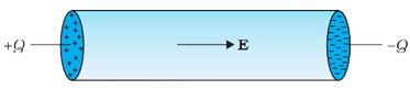
FIGURE 3.1 Charges +Q and –Q put at the ends of a metallic cylinder. The electrons will drift because of the electric field created to neutralise the charges. The current thus will stop after a while unless the charges +Q and –Q are continuously replenished.
Suppose we now take two thin circular discs of a dielectric of the same radius and put positive charge +Q distributed over one disc and similarly –Q at the other disc. We attach the two discs on the two flat surfaces of the cylinder. An electric field will be created and is directed from the positive towards the negative charge. The electrons will be accelerated due to this field towards +Q. They will thus move to neutralise the charges. The electrons, as long as they are moving, will constitute an electric current. Hence in the situation considered, there will be a current for a very short while and no current thereafter.
We can also imagine a mechanism where the ends of the cylinder are supplied with fresh charges to make up for any charges neutralised by electrons moving inside the conductor. In that case, there will be a steady electric field in the body of the conductor. This will result in a continuous current rather than a current for a short period of time. Mechanisms, which maintain a steady electric field are cells or batteries that we shall study later in this chapter. In the next sections, we shall study the steady current that results from a steady electric field in conductors.
OHM’S LAW
A basic law regarding flow of currents was discovered by G.S. Ohm in 1828, long before the physical mechanism responsible for flow of currents was discovered. Imagine a conductor through which a current I is flowing and let V be the potential difference between the ends of the conductor. Then Ohm’s law states that
\(% MathType!MTEF!2!1!+- % feaagKart1ev2aaatCvAUfeBSjuyZL2yd9gzLbvyNv2CaerbuLwBLn % hiov2DGi1BTfMBaeXatLxBI9gBaerbd9wDYLwzYbItLDharqqtubsr % 4rNCHbGeaGqiVu0Je9sqqrpepC0xbbL8F4rqqrFfpeea0xe9Lq-Jc9 % vqaqpepm0xbba9pwe9Q8fs0-yqaqpepae9pg0FirpepeKkFr0xfr-x % fr-xb9adbaqaaeGaciGaaiaabeqaamaabaabaaGceaqabeaacaWGwb % aeaaaaaaaaa8qacqGHDisTcaqGGaGaamysaaqaaiaad+gacaWGYbGa % aiilaiaaykW7caaMc8UaaGPaVlaadAfacqGH9aqpcaWGsbGaamysai % aaykW7caaMc8UaaGPaVlaaykW7caaMc8UaaGPaVlaaykW7caaMc8Ua % aGPaVlaaykW7caaMc8UaaGPaVlaaykW7caaMc8UaaGPaVlaaykW7ca % aMc8UaaGPaVlaaykW7caaMc8UaaGPaVlaaykW7caaMc8UaaGPaVlaa % ykW7daqadaqaaiaaiodacaGGUaGaaG4maaGaayjkaiaawMcaaaaaaa!6EF3! \begin{array}{l} V \propto {\rm{ }}I\\ or,\,\,\,V = RI\,\,\,\,\,\,\,\,\,\,\,\,\,\,\,\,\,\,\,\,\,\,\,\,\,\left( {3.3} \right) \end{array}\)
where the constant of proportionality R is called the resistance of the conductor. The SI units of resistance is ohm, and is denoted by the symbol \(% MathType!MTEF!2!1!+- % feaagKart1ev2aaatCvAUfeBSjuyZL2yd9gzLbvyNv2CaerbuLwBLn % hiov2DGi1BTfMBaeXatLxBI9gBaerbd9wDYLwzYbItLDharqqtubsr % 4rNCHbGeaGqiVu0Je9sqqrpepC0xbbL8F4rqqrFfpeea0xe9Lq-Jc9 % vqaqpepm0xbba9pwe9Q8fs0-yqaqpepae9pg0FirpepeKkFr0xfr-x % fr-xb9adbaqaaeGaciGaaiaabeqaamaabaabaaGcbaaeaaaaaaaaa8 % qacqGHPoWvaaa!37A5! \Omega \). The resistance R not only depends on the material of the conductor but also on the dimensions of the conductor. The dependence of R on the dimensions of the conductor can easily be determined as follows.
Consider a conductor satisfying Eq. (3.3) to be in the form of a slab of length l and cross sectional area A [Fig. 3.2(a)]. Imagine placing two such identical slabs side by side [Fig. 3.2(b)], so that the length of the combination is 2l . The current flowing through the combination is the same as that flowing through either of the slabs. If V is the potential difference across the ends of the first slab, then V is also the potential difference across the ends of the second slab since the second slab is
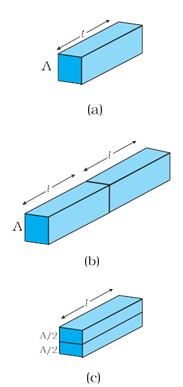
Figure 3.2.
Illustrating the relation R = \(% MathType!MTEF!2!1!+- % feaagKart1ev2aaatCvAUfeBSjuyZL2yd9gzLbvyNv2CaerbuLwBLn % hiov2DGi1BTfMBaeXatLxBI9gBaerbd9wDYLwzYbItLDharqqtubsr % 4rNCHbGeaGqiVu0Je9sqqrpepC0xbbL8F4rqqrFfpeea0xe9Lq-Jc9 % vqaqpepm0xbba9pwe9Q8fs0-yqaqpepae9pg0FirpepeKkFr0xfr-x % fr-xb9adbaqaaeGaciGaaiaabeqaamaabaabaaGcbaaeaaaaaaaaa8 % qacqaHbpGCaaa!37D6! \rho \)l/A for a rectangular slab of length l and area of cross-section A.
identical to the first and the same current I flows through both. The potential difference across the ends of the combination is clearly sum of the potential difference across the two individual slabs and hence equals 2V. The current through the combination is I and the resistance of the combination RC is [from Eq. (3.3)],
\(% MathType!MTEF!2!1!+- % feaagKart1ev2aaatCvAUfeBSjuyZL2yd9gzLbvyNv2CaerbuLwBLn % hiov2DGi1BTfMBaeXatLxBI9gBaerbd9wDYLwzYbItLDharqqtubsr % 4rNCHbGeaGqiVu0Je9sqqrpepC0xbbL8F4rqqrFfpeea0xe9Lq-Jc9 % vqaqpepm0xbba9pwe9Q8fs0-yqaqpepae9pg0FirpepeKkFr0xfr-x % fr-xb9adbaqaaeGaciGaaiaabeqaamaabaabaaGcbaaeaaaaaaaaa8 % qacaWGsbWaaSbaaSqaaiaadoeaaeqaaOGaeyypa0ZaaSaaaeaacaaI % YaGaamOvaaqaaiaadMeaaaGaeyypa0JaaGOmaiaadkfaaaa!3DFF! {R_C} = \frac{{2V}}{I} = 2R\)(3.4)
since V/I = R, the resistance of either of the slabs. Thus, doubling the length of a conductor doubles the resistance. In general, then resistance is proportional to length,
\(% MathType!MTEF!2!1!+- % feaagKart1ev2aaatCvAUfeBSjuyZL2yd9gzLbvyNv2CaerbuLwBLn % hiov2DGi1BTfMBaeXatLxBI9gBaerbd9wDYLwzYbItLDharqqtubsr % 4rNCHbGeaGqiVu0Je9sqqrpepC0xbbL8F4rqqrFfpeea0xe9Lq-Jc9 % vqaqpepm0xbba9pwe9Q8fs0-yqaqpepae9pg0FirpepeKkFr0xfr-x % fr-xb9adbaqaaeGaciGaaiaabeqaamaabaabaaGcbaaeaaaaaaaaa8 % qacaWGsbGaeyyhIuRaamiBaaaa!395E! R \propto l\) (3.5)
Next, imagine dividing the slab into two by cutting it lengthwise so that the slab can be considered as a combination of two identical slabs of length l , but each having a cross sectional area of A/2 [Fig. 3.2(c)].
For a given voltage V across the slab, if I is the current through the entire slab, then clearly the current flowing through each of the two half-slabs is I/2. Since the potential difference across the ends of the half-slabs is V, i.e., the same as across the full slab, the resistance of each of the half-slabs R1 is
\(% MathType!MTEF!2!1!+- % feaagKart1ev2aaatCvAUfeBSjuyZL2yd9gzLbvyNv2CaerbuLwBLn % hiov2DGi1BTfMBaeXatLxBI9gBaerbd9wDYLwzYbItLDharqqtubsr % 4rNCHbGeaGqiVu0Je9sqqrpepC0xbbL8F4rqqrFfpeea0xe9Lq-Jc9 % vqaqpepm0xbba9pwe9Q8fs0-yqaqpepae9pg0FirpepeKkFr0xfr-x % fr-xb9adbaqaaeGaciGaaiaabeqaamaabaabaaGcbaGaamOuamaaBa % aaleaacaaIXaaabeaakiabg2da9maalaaabaGaamOvaaqaaiaadMea % caGGVaGaaGOmaaaacqGH9aqpcaaIYaWaaSaaaeaacaWGwbaabaGaam % ysaaaacqGH9aqpcaaIYaGaamOuaaaa!4200! {R_1} = \frac{V}{{I/2}} = 2\frac{V}{I} = 2R\)(3.6)
Thus, halving the area of the cross-section of a conductor doubles the resistance. In general, then the resistance R is inversely proportional to the cross-sectional area,
\(% MathType!MTEF!2!1!+- % feaagKart1ev2aaatCvAUfeBSjuyZL2yd9gzLbvyNv2CaerbuLwBLn % hiov2DGi1BTfMBaeXatLxBI9gBaerbd9wDYLwzYbItLDharqqtubsr % 4rNCHbGeaGqiVu0Je9sqqrpepC0xbbL8F4rqqrFfpeea0xe9Lq-Jc9 % vqaqpepm0xbba9pwe9Q8fs0-yqaqpepae9pg0FirpepeKkFr0xfr-x % fr-xb9adbaqaaeGaciGaaiaabeqaamaabaabaaGcbaaeaaaaaaaaa8 % qacaWGsbGaeyyhIu7aaSaaaeaacaaIXaaabaGaamyqaaaaaaa!39FE! R \propto \frac{1}{A}\) (3.7)
Combining Eqs. (3.5) and (3.7), we have
\(% MathType!MTEF!2!1!+- % feaagKart1ev2aaatCvAUfeBSjuyZL2yd9gzLbvyNv2CaerbuLwBLn % hiov2DGi1BTfMBaeXatLxBI9gBaerbd9wDYLwzYbItLDharqqtubsr % 4rNCHbGeaGqiVu0Je9sqqrpepC0xbbL8F4rqqrFfpeea0xe9Lq-Jc9 % vqaqpepm0xbba9pwe9Q8fs0-yqaqpepae9pg0FirpepeKkFr0xfr-x % fr-xb9adbaqaaeGaciGaaiaabeqaamaabaabaaGcbaaeaaaaaaaaa8 % qacaWGsbGaeyyhIu7aaSaaaeaacaaIXaaabaGaamyqaaaaaaa!39FE! R \propto \frac{1}{A}\) (3.8)
and hence for a given conductor
\(% MathType!MTEF!2!1!+- % feaagKart1ev2aaatCvAUfeBSjuyZL2yd9gzLbvyNv2CaerbuLwBLn % hiov2DGi1BTfMBaeXatLxBI9gBaerbd9wDYLwzYbItLDharqqtubsr % 4rNCHbGeaGqiVu0Je9sqqrpepC0xbbL8F4rqqrFfpeea0xe9Lq-Jc9 % vqaqpepm0xbba9pwe9Q8fs0-yqaqpepae9pg0FirpepeKkFr0xfr-x % fr-xb9adbaqaaeGaciGaaiaabeqaamaabaabaaGcbaaeaaaaaaaaa8 % qacaWGsbGaeyypa0JaeqyWdi3aaSaaaeaacaWGSbaabaGaamyqaaaa % aaa!3B7A! R = \rho \frac{l}{A}\) (3.9)
where the constant of proportionality \(% MathType!MTEF!2!1!+- % feaagKart1ev2aaatCvAUfeBSjuyZL2yd9gzLbvyNv2CaerbuLwBLn % hiov2DGi1BTfMBaeXatLxBI9gBaerbd9wDYLwzYbItLDharqqtubsr % 4rNCHbGeaGqiVu0Je9sqqrpepC0xbbL8F4rqqrFfpeea0xe9Lq-Jc9 % vqaqpepm0xbba9pwe9Q8fs0-yqaqpepae9pg0FirpepeKkFr0xfr-x % fr-xb9adbaqaaeGaciGaaiaabeqaamaabaabaaGcbaaeaaaaaaaaa8 % qacqaHbpGCaaa!37D6! \rho \) depends on the material of the conductor but not on its dimensions. \(% MathType!MTEF!2!1!+- % feaagKart1ev2aaatCvAUfeBSjuyZL2yd9gzLbvyNv2CaerbuLwBLn % hiov2DGi1BTfMBaeXatLxBI9gBaerbd9wDYLwzYbItLDharqqtubsr % 4rNCHbGeaGqiVu0Je9sqqrpepC0xbbL8F4rqqrFfpeea0xe9Lq-Jc9 % vqaqpepm0xbba9pwe9Q8fs0-yqaqpepae9pg0FirpepeKkFr0xfr-x % fr-xb9adbaqaaeGaciGaaiaabeqaamaabaabaaGcbaaeaaaaaaaaa8 % qacqaHbpGCaaa!37D6! \rho \) is called resistivity.
Using the last equation, Ohm’s law reads
\(% MathType!MTEF!2!1!+- % feaagKart1ev2aaatCvAUfeBSjuyZL2yd9gzLbvyNv2CaerbuLwBLn % hiov2DGi1BTfMBaeXatLxBI9gBaerbd9wDYLwzYbItLDharqqtubsr % 4rNCHbGeaGqiVu0Je9sqqrpepC0xbbL8F4rqqrFfpeea0xe9Lq-Jc9 % vqaqpepm0xbba9pwe9Q8fs0-yqaqpepae9pg0FirpepeKkFr0xfr-x % fr-xb9adbaqaaeGaciGaaiaabeqaamaabaabaaGcbaGaamOvaiabg2 % da9iaadMeacqGHxdaTcaWGsbGaeyypa0ZaaSaaaeaacaWGjbGaeqyW % diNaamiBaaqaaiaadgeaaaaaaa!40EE! V = I \times R = \frac{{I\rho l}}{A}\) (3.10)
Current per unit area (taken normal to the current), I/A, is called current density and is denoted by j. The SI units of the current density are A/m2. Further, if E is the magnitude of uniform electric field in the conductor whose length is l, then the potential difference V across its ends is El. Using these, the last equation reads
E l = j \(% MathType!MTEF!2!1!+- % feaagKart1ev2aaatCvAUfeBSjuyZL2yd9gzLbvyNv2CaerbuLwBLn % hiov2DGi1BTfMBaeXatLxBI9gBaerbd9wDYLwzYbItLDharqqtubsr % 4rNCHbGeaGqiVu0Je9sqqrpepC0xbbL8F4rqqrFfpeea0xe9Lq-Jc9 % vqaqpepm0xbba9pwe9Q8fs0-yqaqpepae9pg0FirpepeKkFr0xfr-x % fr-xb9adbaqaaeGaciGaaiaabeqaamaabaabaaGcbaGaeqyWdihaaa!37B6! \rho \) l
or, E = j \(% MathType!MTEF!2!1!+- % feaagKart1ev2aaatCvAUfeBSjuyZL2yd9gzLbvyNv2CaerbuLwBLn % hiov2DGi1BTfMBaeXatLxBI9gBaerbd9wDYLwzYbItLDharqqtubsr % 4rNCHbGeaGqiVu0Je9sqqrpepC0xbbL8F4rqqrFfpeea0xe9Lq-Jc9 % vqaqpepm0xbba9pwe9Q8fs0-yqaqpepae9pg0FirpepeKkFr0xfr-x % fr-xb9adbaqaaeGaciGaaiaabeqaamaabaabaaGcbaGaeqyWdihaaa!37B6! \rho \) (3.11)
The above relation for magnitudes E and j can indeed be cast in a vector form. The current density, (which we have defined as the current through unit area normal to the current) is also directed along E, and is also a vector j (\(% MathType!MTEF!2!1!+- % feaagKart1ev2aaatCvAUfeBSjuyZL2yd9gzLbvyNv2CaerbuLwBLn % hiov2DGi1BTfMBaeXatLxBI9gBaerbd9wDYLwzYbItLDharqqtubsr % 4rNCHbGeaGqiVu0Je9sqqrpepC0xbbL8F4rqqrFfpeea0xe9Lq-Jc9 % vqaqpepm0xbba9pwe9Q8fs0-yqaqpepae9pg0FirpepeKkFr0xfr-x % fr-xb9adbaqaaeGaciGaaiaabeqaamaabaabaaGcbaGaeyyyIOlaaa!37BF! \equiv \) j E/E). Thus, the last equation can be written as,
\(% MathType!MTEF!2!1!+- % feaagKart1ev2aaatCvAUfeBSjuyZL2yd9gzLbvyNv2CaerbuLwBLn % hiov2DGi1BTfMBaeXatLxBI9gBaerbd9wDYLwzYbItLDharqqtubsr % 4rNCHbGeaGqiVu0Je9sqqrpepC0xbbL8F4rqqrFfpeea0xe9Lq-Jc9 % vqaqpepm0xbba9pwe9Q8fs0-yqaqpepae9pg0FirpepeKkFr0xfr-x % fr-xb9adbaqaaeGaciGaaiaabeqaamaabaabaaGceaqabeaacaWGfb % Gaeyypa0JaamOAaiabeg8aYjaaykW7caaMc8UaaGPaVlaaykW7caaM % c8UaaGPaVlaaykW7caaMc8UaaGPaVlaaykW7caaMc8UaaGPaVlaayk % W7caaMc8UaaGPaVlaaykW7caaMc8UaaGPaVlaaykW7caaMc8+aaeWa % aeaacaaIZaGaaiOlaiaaigdacaaIYaaacaGLOaGaayzkaaGaaGPaVl % aaykW7caaMc8UaaGPaVlaaykW7caaMc8UaaGPaVlaaykW7caaMc8Ua % aGPaVlaaykW7aeaacaWGVbGaamOCaiaacYcacaaMc8UaaGPaVlaadQ % gacqGH9aqpcqaHdpWCcaWGfbGaaGPaVlaaykW7caaMc8UaaGPaVlaa % ykW7caaMc8UaaGPaVlaaykW7caaMc8UaaGPaVlaacIcacaaIZaGaai % OlaiaaigdacaaIZaGaaiykaaaaaa!8CA1! \begin{array}{l} E = j\rho \,\,\,\,\,\,\,\,\,\,\,\,\,\,\,\,\,\,\,\,\left( {3.12} \right)\,\,\,\,\,\,\,\,\,\,\,\\ or,\,\,j = \sigma E\,\,\,\,\,\,\,\,\,\,(3.13) \end{array}\)
where \(% MathType!MTEF!2!1!+- % feaagKart1ev2aaatCvAUfeBSjuyZL2yd9gzLbvyNv2CaerbuLwBLn % hiov2DGi1BTfMBaeXatLxBI9gBaerbd9wDYLwzYbItLDharqqtubsr % 4rNCHbGeaGqiVu0Je9sqqrpepC0xbbL8F4rqqrFfpeea0xe9Lq-Jc9 % vqaqpepm0xbba9pwe9Q8fs0-yqaqpepae9pg0FirpepeKkFr0xfr-x % fr-xb9adbaqaaeGaciGaaiaabeqaamaabaabaaGcbaGaeq4WdmNaey % yyIORaaGymaiaac+cacqaHbpGCaaa!3CB0! \sigma \equiv 1/\rho \) is called the conductivity. Ohm’s law is often stated in an equivalent form, Eq. (3.13) in addition to Eq.(3.3). In the next section, we will try to understand the origin of the Ohm’s law as arising from the characteristics of the drift of electrons.
DRIFT DRIFT OF ELECTRONS AND THE ORIGIN OF RESISTIVITY
As remarked before, an electron will suffer collisions with the heavy fixed ions, but after collision, it will emerge with the same speed but in random directions. If we consider all the electrons, their average velocity will be zero since their directions are random. Thus, if there are N electrons and the velocity of the ith electron (i = 1, 2, 3, ... N ) at a given time is vi , then
\(% MathType!MTEF!2!1!+- % feaagKart1ev2aaatCvAUfeBSjuyZL2yd9gzLbvyNv2CaerbuLwBLn % hiov2DGi1BTfMBaeXatLxBI9gBaerbd9wDYLwzYbItLDharqqtubsr % 4rNCHbGeaGqiVu0Je9sqqrpepC0xbbL8F4rqqrFfpeea0xe9Lq-Jc9 % vqaqpepm0xbba9pwe9Q8fs0-yqaqpepae9pg0FirpepeKkFr0xfr-x % fr-xb9adbaqaaeGaciGaaiaabeqaamaabaabaaGcbaWaaSaaaeaaca % aIXaaabaGaamOtaaaadaaeWbqaaiaadAhadaWgaaWcbaGaamyAaaqa % baaabaGaamyAaiabg2da9iaaigdaaeaacaWGobaaniabggHiLdGccq % GH9aqpcaaIWaaaaa!412C! \frac{1}{N}\sum\limits_{i = 1}^N {{v_i}} = 0\)(3.14)
Consider now the situation when an electric field is present. Electrons will be accelerated due to this field by
\(% MathType!MTEF!2!1!+- % feaagKart1ev2aaatCvAUfeBSjuyZL2yd9gzLbvyNv2CaerbuLwBLn % hiov2DGi1BTfMBaeXatLxBI9gBaerbd9wDYLwzYbItLDharqqtubsr % 4rNCHbGeaGqiVu0Je9sqqrpepC0xbbL8F4rqqrFfpeea0xe9Lq-Jc9 % vqaqpepm0xbba9pwe9Q8fs0-yqaqpepae9pg0FirpepeKkFr0xfr-x % fr-xb9adbaqaaeGaciGaaiaabeqaamaabaabaaGcbaGaamyyaiabg2 % da9maalaaabaGaeyOeI0IaamyzaiaadweaaeaacaWGTbaaaaaa!3B85! a = \frac{{ - eE}}{m}\) (3.15)
where –e is the charge and m is the mass of an electron. Consider again the ith electron at a given time t. This electron would have had its last collision some time before t, and let ti be the time elapsed after its last collision. If vi was its velocity immediately after the last collision, then its velocity Vi at time t is
\(% MathType!MTEF!2!1!+- % feaagKart1ev2aaatCvAUfeBSjuyZL2yd9gzLbvyNv2CaerbuLwBLn % hiov2DGi1BTfMBaeXatLxBI9gBaerbd9wDYLwzYbItLDharqqtubsr % 4rNCHbGeaGqiVu0Je9sqqrpepC0xbbL8F4rqqrFfpeea0xe9Lq-Jc9 % vqaqpepm0xbba9pwe9Q8fs0-yqaqpepae9pg0FirpepeKkFr0xfr-x % fr-xb9adbaqaaeGaciGaaiaabeqaamaabaabaaGcbaGaamOvamaaBa % aaleaacaWGPbaabeaakiabg2da9iaadAhadaWgaaWcbaGaamyAaaqa % baGccqGHRaWkdaWcaaqaaiaadwgacaWGfbaabaGaamyBaaaacaWG0b % WaaSbaaSqaaiaadMgaaeqaaaaa!40C5! {V_i} = {v_i} + \frac{{eE}}{m}{t_i}\)(3.16)
since starting with its last collision it was accelerated (Fig. 3.3) with an acceleration given by Eq. (3.15) for a time interval ti . The average velocity of the electrons at time t is the average of all the Vi’s. The average of vi’s is
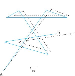
FIGURE 3.3 A schematic picture of an electron moving from a point A to another point B through repeated collisions, and straight line travel between collisions (full lines). If an electric field is applied as shown, the electron ends up at point \(% MathType!MTEF!2!1!+- % feaagKart1ev2aaatCvAUfeBSjuyZL2yd9gzLbvyNv2CaerbuLwBLn % hiov2DGi1BTfMBaeXatLxBI9gBaerbd9wDYLwzYbItLDharqqtubsr % 4rNCHbGeaGqiVu0Je9sqqrpepC0xbbL8F4rqqrFfpeea0xe9Lq-Jc9 % vqaqpepm0xbba9pwe9Q8fs0-yqaqpepae9pg0FirpepeKkFr0xfr-x % fr-xb9adbaqaaeGaciGaaiaabeqaamaabaabaaGcbaGabmOqayaafa % aaaa!36C9! B'\) (dotted lines). A slight drift in a direction opposite the electric field is visible.
time more than \(% MathType!MTEF!2!1!+- % feaagKart1ev2aaatCvAUfeBSjuyZL2yd9gzLbvyNv2CaerbuLwBLn % hiov2DGi1BTfMBaeXatLxBI9gBaerbd9wDYLwzYbItLDharqqtubsr % 4rNCHbGeaGqiVu0Je9sqqrpepC0xbbL8F4rqqrFfpeea0xe9Lq-Jc9 % vqaqpepm0xbba9pwe9Q8fs0-yqaqpepae9pg0FirpepeKkFr0xfr-x % fr-xb9adbaqaaeGaciGaaiaabeqaamaabaabaaGcbaGaeqiXdqhaaa!37BB! \tau \) and some less than \(% MathType!MTEF!2!1!+- % feaagKart1ev2aaatCvAUfeBSjuyZL2yd9gzLbvyNv2CaerbuLwBLn % hiov2DGi1BTfMBaeXatLxBI9gBaerbd9wDYLwzYbItLDharqqtubsr % 4rNCHbGeaGqiVu0Je9sqqrpepC0xbbL8F4rqqrFfpeea0xe9Lq-Jc9 % vqaqpepm0xbba9pwe9Q8fs0-yqaqpepae9pg0FirpepeKkFr0xfr-x % fr-xb9adbaqaaeGaciGaaiaabeqaamaabaabaaGcbaGaeqiXdqhaaa!37BB! \tau \). In other words, the time t in Eq. (3.16) will be less than \(% MathType!MTEF!2!1!+- % feaagKart1ev2aaatCvAUfeBSjuyZL2yd9gzLbvyNv2CaerbuLwBLn % hiov2DGi1BTfMBaeXatLxBI9gBaerbd9wDYLwzYbItLDharqqtubsr % 4rNCHbGeaGqiVu0Je9sqqrpepC0xbbL8F4rqqrFfpeea0xe9Lq-Jc9 % vqaqpepm0xbba9pwe9Q8fs0-yqaqpepae9pg0FirpepeKkFr0xfr-x % fr-xb9adbaqaaeGaciGaaiaabeqaamaabaabaaGcbaGaeqiXdqhaaa!37BB! \tau \) for some and more than \(% MathType!MTEF!2!1!+- % feaagKart1ev2aaatCvAUfeBSjuyZL2yd9gzLbvyNv2CaerbuLwBLn % hiov2DGi1BTfMBaeXatLxBI9gBaerbd9wDYLwzYbItLDharqqtubsr % 4rNCHbGeaGqiVu0Je9sqqrpepC0xbbL8F4rqqrFfpeea0xe9Lq-Jc9 % vqaqpepm0xbba9pwe9Q8fs0-yqaqpepae9pg0FirpepeKkFr0xfr-x % fr-xb9adbaqaaeGaciGaaiaabeqaamaabaabaaGcbaGaeqiXdqhaaa!37BB! \tau \) for others as we go through the values of i = 1, 2 ..... N. The average value of ti then is \(% MathType!MTEF!2!1!+- % feaagKart1ev2aaatCvAUfeBSjuyZL2yd9gzLbvyNv2CaerbuLwBLn % hiov2DGi1BTfMBaeXatLxBI9gBaerbd9wDYLwzYbItLDharqqtubsr % 4rNCHbGeaGqiVu0Je9sqqrpepC0xbbL8F4rqqrFfpeea0xe9Lq-Jc9 % vqaqpepm0xbba9pwe9Q8fs0-yqaqpepae9pg0FirpepeKkFr0xfr-x % fr-xb9adbaqaaeGaciGaaiaabeqaamaabaabaaGcbaGaeqiXdqhaaa!37BB! \tau \) (known as relaxation time). Thus, averaging Eq. (3.16) over the
\(% MathType!MTEF!2!1!+- % feaagKart1ev2aaatCvAUfeBSjuyZL2yd9gzLbvyNv2CaerbuLwBLn % hiov2DGi1BTfMBaeXatLxBI9gBaerbd9wDYLwzYbItLDharqqtubsr % 4rNCHbGeaGqiVu0Je9sqqrpepC0xbbL8F4rqqrFfpeea0xe9Lq-Jc9 % vqaqpepm0xbba9pwe9Q8fs0-yqaqpepae9pg0FirpepeKkFr0xfr-x % fr-xb9adbaqaaeGaciGaaiaabeqaamaabaabaaGceaqabeaacaWG2b % WaaSbaaSqaaiaadsgaaeqaaOGaeyypa0ZaaeWaaeaacaWGwbWaaSba % aSqaaiaadMgaaeqaaaGccaGLOaGaayzkaaWaaSbaaSqaaiaadggaca % WG2bGaamyzaiaadkhacaWGHbGaam4zaiaadwgaaeqaaOGaeyOeI0Ya % aSaaaeaacaWGLbGaamyraaqaaiaad2gaaaWaaeWaaeaacaWG0bWaaS % baaSqaaiaadMgaaeqaaaGccaGLOaGaayzkaaWaaSbaaSqaaiaadgga % caWG2bGaamyzaiaadkhacaWGHbGaam4zaiaadwgaaeqaaaGcbaGaey % ypa0JaaGimaiabgkHiTmaalaaabaGaamyzaiaadweaaeaacaWGTbaa % aiabes8a0jabg2da9iabgkHiTmaalaaabaGaamyzaiaadweaaeaaca % WGTbaaaiabes8a0jaaykW7caaMc8UaaGPaVlaaykW7caaMc8UaaGPa % VlaaykW7caaMc8UaaGPaVlaaykW7caaMc8UaaGPaVlaaykW7caaMc8 % UaaGPaVlaaykW7caaMc8UaaGPaVlaaykW7caaMc8UaaGPaVpaabmaa % baGaaG4maiaac6cacaaIXaGaaG4naaGaayjkaiaawMcaaaaaaa!83C7! \begin{array}{l} {v_d} = {\left( {{V_i}} \right)_{average}} - \frac{{eE}}{m}{\left( {{t_i}} \right)_{average}}\\ = 0 - \frac{{eE}}{m}\tau = - \frac{{eE}}{m}\tau \,\,\,\,\,\,\,\,\,\,\,\,\,\,\,\,\,\,\,\,\,\left( {3.17} \right) \end{array}\)
This last result is surprising. It tells us that the electrons move with an average velocity which is independent of time, although electrons are accelerated. This is the phenomenon of drift and the velocity vd in Eq. (3.17) is called the drift velocity.
Because of the drift, there will be net transport of charges across any area perpendicular to E. Consider a planar area A, located inside the conductor such that the normal to the area is parallel to E (Fig. 3.4).
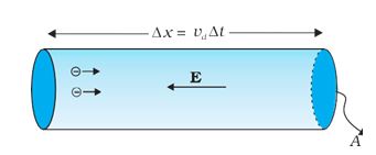
FIGURE 3.4 Current in a metallic conductor. The magnitude of current density in a metal is the magnitude of charge contained in a cylinder of unit area and length vd.
because of the drift, in an infinitesimal amount of time \(\Delta\)t, all electrons to the left of the area at distances upto |vd|\(\Delta\)t would have crossed the area. If n is the number of free electrons per unit volume in the metal, then there are n \(\Delta\)t |vd|A such electrons. Since each electron carries a charge –e, the total charge transported across this area A to the right in time \(\Delta\)t is –ne A|vd|\(\Delta\)t. E is directed towards the left and hence the total charge transported along E across the area is negative of this. The amount of charge crossing the area A in time \(\Delta\)t is by definition [Eq. (3.2)] I \(\Delta\)t, where I is the magnitude of the current. Hence,
\(% MathType!MTEF!2!1!+- % feaagKart1ev2aaatCvAUfeBSjuyZL2yd9gzLbvyNv2CaerbuLwBLn % hiov2DGi1BTfMBaeXatLxBI9gBaerbd9wDYLwzYbItLDharqqtubsr % 4rNCHbGeaGqiVu0Je9sqqrpepC0xbbL8F4rqqrFfpeea0xe9Lq-Jc9 % vqaqpepm0xbba9pwe9Q8fs0-yqaqpepae9pg0FirpepeKkFr0xfr-x % fr-xb9adbaqaaeGaciGaaiaabeqaamaabaabaaGcbaGaamysaiabgs % 5aejaadshacqGH9aqpcqGHRaWkcaWGUbGaamyzaiaadgeadaabdaqa % aiaadAhadaWgaaWcbaGaamizaaqabaaakiaawEa7caGLiWoacqGHuo % arcaWG0baaaa!454B! I\Delta t = + neA\left| {{v_d}} \right|\Delta t\) (3.18)
Substituting the value of \(% MathType!MTEF!2!1!+- % feaagKart1ev2aaatCvAUfeBSjuyZL2yd9gzLbvyNv2CaerbuLwBLn % hiov2DGi1BTfMBaeXatLxBI9gBaerbd9wDYLwzYbItLDharqqtubsr % 4rNCHbGeaGqiVu0Je9sqqrpepC0xbbL8F4rqqrFfpeea0xe9Lq-Jc9 % vqaqpepm0xbba9pwe9Q8fs0-yqaqpepae9pg0FirpepeKkFr0xfr-x % fr-xb9adbaqaaeGaciGaaiaabeqaamaabaabaaGcbaWaaqWaaeaaca % WG2bWaaSbaaSqaaiaadsgaaeqaaaGccaGLhWUaayjcSdGaeyiLdqKa % amiDaaaa!3D92! \left| {{v_d}} \right|\Delta t\) from Eq. (3.17)
\(% MathType!MTEF!2!1!+- % feaagKart1ev2aaatCvAUfeBSjuyZL2yd9gzLbvyNv2CaerbuLwBLn % hiov2DGi1BTfMBaeXatLxBI9gBaerbd9wDYLwzYbItLDharqqtubsr % 4rNCHbGeaGqiVu0Je9sqqrpepC0xbbL8F4rqqrFfpeea0xe9Lq-Jc9 % vqaqpepm0xbba9pwe9Q8fs0-yqaqpepae9pg0FirpepeKkFr0xfr-x % fr-xb9adbaqaaeGaciGaaiaabeqaamaabaabaaGcbaGaamysaiabgs % 5aejaadshacqGH9aqpdaWcaaqaaiaadwgadaahaaWcbeqaaiaaikda % aaGccaWGbbaabaGaamyBaaaacqaHepaDcaWGUbGaey4bIeTaamiDam % aaemaabaGaamyraaGaay5bSlaawIa7aaaa!46F2! I\Delta t = \frac{{{e^2}A}}{m}\tau n\nabla t\left| E \right|\)(3.19)
By definition I is related to the magnitude |j| of the current density by
\(% MathType!MTEF!2!1!+- % feaagKart1ev2aaatCvAUfeBSjuyZL2yd9gzLbvyNv2CaerbuLwBLn % hiov2DGi1BTfMBaeXatLxBI9gBaerbd9wDYLwzYbItLDharqqtubsr % 4rNCHbGeaGqiVu0Je9sqqrpepC0xbbL8F4rqqrFfpeea0xe9Lq-Jc9 % vqaqpepm0xbba9pwe9Q8fs0-yqaqpepae9pg0FirpepeKkFr0xfr-x % fr-xb9adbaqaaeGaciGaaiaabeqaamaabaabaaGcbaGaamysaiabg2 % da9maaemaabaGaamOAaaGaay5bSlaawIa7aiaadgeaaaa!3CA1! I = \left| j \right|A\) (3.20)
Hence, from Eqs.(3.19) and (3.20),
\(% MathType!MTEF!2!1!+- % feaagKart1ev2aaatCvAUfeBSjuyZL2yd9gzLbvyNv2CaerbuLwBLn % hiov2DGi1BTfMBaeXatLxBI9gBaerbd9wDYLwzYbItLDharqqtubsr % 4rNCHbGeaGqiVu0Je9sqqrpepC0xbbL8F4rqqrFfpeea0xe9Lq-Jc9 % vqaqpepm0xbba9pwe9Q8fs0-yqaqpepae9pg0FirpepeKkFr0xfr-x % fr-xb9adbaqaaeGaciGaaiaabeqaamaabaabaaGcbaWaaqWaaeaaca % WGQbaacaGLhWUaayjcSdGaeyypa0ZaaSaaaeaacaWGUbGaamyzamaa % CaaaleqabaGaaGOmaaaaaOqaaiaad2gaaaGaeqiXdq3aaqWaaeaaca % WGfbaacaGLhWUaayjcSdaaaa!4490! \left| j \right| = \frac{{n{e^2}}}{m}\tau \left| E \right|\)(3.21)
The vector j is parallel to E and hence we can write Eq. (3.21) in the vector form
\(% MathType!MTEF!2!1!+- % feaagKart1ev2aaatCvAUfeBSjuyZL2yd9gzLbvyNv2CaerbuLwBLn % hiov2DGi1BTfMBaeXatLxBI9gBaerbd9wDYLwzYbItLDharqqtubsr % 4rNCHbGeaGqiVu0Je9sqqrpepC0xbbL8F4rqqrFfpeea0xe9Lq-Jc9 % vqaqpepm0xbba9pwe9Q8fs0-yqaqpepae9pg0FirpepeKkFr0xfr-x % fr-xb9adbaqaaeGaciGaaiaabeqaamaabaabaaGcbaGaamOAaiabg2 % da9maalaaabaGaamOBaiaadwgadaahaaWcbeqaaiaaikdaaaaakeaa % caWGTbaaaiabes8a0jaadweaaaa!3E4C! j = \frac{{n{e^2}}}{m}\tau E\)(3.22)
Comparison with Eq. (3.13) shows that Eq. (3.22) is exactly the Ohm’s law, if we identify the conductivity \(% MathType!MTEF!2!1!+- % feaagKart1ev2aaatCvAUfeBSjuyZL2yd9gzLbvyNv2CaerbuLwBLn % hiov2DGi1BTfMBaeXatLxBI9gBaerbd9wDYLwzYbItLDharqqtubsr % 4rNCHbGeaGqiVu0Je9sqqrpepC0xbbL8F4rqqrFfpeea0xe9Lq-Jc9 % vqaqpepm0xbba9pwe9Q8fs0-yqaqpepae9pg0FirpepeKkFr0xfr-x % fr-xb9adbaqaaeGaciGaaiaabeqaamaabaabaaGcbaGaeq4Wdmhaaa!37B9! \sigma \) as
\(% MathType!MTEF!2!1!+- % feaagKart1ev2aaatCvAUfeBSjuyZL2yd9gzLbvyNv2CaerbuLwBLn % hiov2DGi1BTfMBaeXatLxBI9gBaerbd9wDYLwzYbItLDharqqtubsr % 4rNCHbGeaGqiVu0Je9sqqrpepC0xbbL8F4rqqrFfpeea0xe9Lq-Jc9 % vqaqpepm0xbba9pwe9Q8fs0-yqaqpepae9pg0FirpepeKkFr0xfr-x % fr-xb9adbaqaaeGaciGaaiaabeqaamaabaabaaGcbaGaeq4WdmNaey % ypa0ZaaSaaaeaacaWGUbGaamyzamaaCaaaleqabaGaaGOmaaaaaOqa % aiaad2gaaaGaamOCaaaa!3D88! \sigma = \frac{{n{e^2}}}{m}r\)(3.23)
We thus see that a very simple picture of electrical conduction reproduces Ohm’s law. We have, of course, made assumptions that \(% MathType!MTEF!2!1!+- % feaagKart1ev2aaatCvAUfeBSjuyZL2yd9gzLbvyNv2CaerbuLwBLn % hiov2DGi1BTfMBaeXatLxBI9gBaerbd9wDYLwzYbItLDharqqtubsr % 4rNCHbGeaGqiVu0Je9sqqrpepC0xbbL8F4rqqrFfpeea0xe9Lq-Jc9 % vqaqpepm0xbba9pwe9Q8fs0-yqaqpepae9pg0FirpepeKkFr0xfr-x % fr-xb9adbaqaaeGaciGaaiaabeqaamaabaabaaGcbaGaeqiXdqhaaa!37BB! \tau \) and n are constants, independent of E. We shall, in the next section, discuss the limitations of Ohm’s law.
EXAMPLE 1
(a) Estimate the average drift speed of conduction electrons in a copper wire of cross-sectional area 1.0 × 10⁻⁷ m2 carrying a current of 1.5 A. Assume that each copper atom contributes roughly one conduction electron. The density of copper is 9.0 × 10³ kg/m3, and its atomic mass is 63.5 u. (b) Compare the drift speed obtained above with, (i) thermal speeds of copper atoms at ordinary temperatures, (ii) speed of propagation of electric field along the conductor which causes the drift motion.
SOLUTION
a. The direction of drift velocity of conduction electrons is opposite to the electric field direction, i.e., electrons drift in the direction of increasing potential. The drift speed vd is given by Eq. (3.18)
\(v_d\) = (I/neA)
Now, e = 1.6 × 10⁻¹⁹ C, A = 1.0 × 10⁻⁷m2, I = 1.5 A. The density of conduction electrons, n is equal to the number of atoms per cubic metre (assuming one conduction electron per Cu atom as is reasonable from its valence electron count of one). A cubic metre of copper has a mass of 9.0 × 10³ kg. Since 6.0 × 10²³ copper atoms have a mass of 63.5 g,
\(% MathType!MTEF!2!1!+- % feaagKart1ev2aaatCvAUfeBSjuyZL2yd9gzLbvyNv2CaerbuLwBLn % hiov2DGi1BTfMBaeXatLxBI9gBaerbd9wDYLwzYbItLDharqqtubsr % 4rNCHbGeaGqiVu0Je9sqqrpepC0xbbL8F4rqqrFfpeea0xe9Lq-Jc9 % vqaqpepm0xbba9pwe9Q8fs0-yqaqpepae9pg0FirpepeKkFr0xfr-x % fr-xb9adbaqaaeGaciGaaiaabeqaamaabaabaaGceaqabeaacaWGUb % Gaeyypa0ZaaSaaaeaacaaI2aGaaiOlaiaaicdacqGHxdaTcaaIXaGa % aGimamaaCaaaleqabaGaaGOmaiaaiodaaaaakeaacaaI2aGaaG4mai % aac6cacaaI1aaaaiabgEna0kaaiMdacaGGUaGaaGimaiabgEna0kaa % igdacaaIWaWaaWbaaSqabeaacaaI2aaaaaGcbaGaeyypa0JaaGioai % aac6cacaaI1aGaey41aqRaaGymaiaaicdadaahaaWcbeqaaiaaikda % caaI4aaaaOGaamyBamaaCaaaleqabaGaeyOeI0IaaG4maaaaaaaa!5668! \begin{array}{l} n = \frac{{6.0 \times {{10}^{23}}}}{{63.5}} \times 9.0 \times {10^6}\\ = 8.5 \times {10^{28}}{m^{ - 3}} \end{array}\)
which given,
\(% MathType!MTEF!2!1!+- % feaagKart1ev2aaatCvAUfeBSjuyZL2yd9gzLbvyNv2CaerbuLwBLn % hiov2DGi1BTfMBaeXatLxBI9gBaerbd9wDYLwzYbItLDharqqtubsr % 4rNCHbGeaGqiVu0Je9sqqrpepC0xbbL8F4rqqrFfpeea0xe9Lq-Jc9 % vqaqpepm0xbba9pwe9Q8fs0-yqaqpepae9pg0FirpepeKkFr0xfr-x % fr-xb9adbaqaaeGaciGaaiaabeqaamaabaabaaGceaqabeaacaWG2b % WaaSbaaSqaaiaadsgaaeqaaOGaeyypa0ZaaSaaaeaacaaIXaGaaiOl % aiaaiwdaaeaacaaI4aGaaiOlaiaaiwdacqGHxdaTcaaIXaGaaGimam % aaCaaaleqabaGaaGOmaiaaiIdaaaGccqGHxdaTcaaIXaGaaiOlaiaa % iAdacqGHxdaTcaaIXaGaaGimamaaCaaaleqabaGaeyOeI0IaaGymai % aaiMdaaaGccqGHxdaTcaaIXaGaaiOlaiaaicdacqGHxdaTcaaIXaGa % aGimamaaCaaaleqabaGaeyOeI0IaaG4naaaaaaaakeaacqGH9aqpca % aIXaGaaiOlaiaaigdacqGHxdaTcaaIXaGaaGimamaaCaaaleqabaGa % eyOeI0IaaG4maaaakiaad2gacaWGZbWaaWbaaSqabeaacqGHsislca % aIXaaaaOGaeyypa0JaaGymaiaac6cacaaIXaGaamyBaiaad2gacaWG % ZbGaamiAamaaCaaaleqabaGaeyOeI0IaaGymaaaaaaaa!6C1E! \begin{array}{l} {v_d} = \frac{{1.5}}{{8.5 \times {{10}^{28}} \times 1.6 \times {{10}^{ - 19}} \times 1.0 \times {{10}^{ - 7}}}}\\ = 1.1 \times {10^{ - 3}}m{s^{ - 1}} = 1.1mms{h^{ - 1}} \end{array}\)
b. (i) At a temperature T, the thermal speed* of a copper atom of mass M is obtained from [<(1/2) Mv2 > = (3/2) kBT ] and is thustypically of the order of \(% MathType!MTEF!2!1!+- % feaagKart1ev2aaatCvAUfeBSjuyZL2yd9gzLbvyNv2CaerbuLwBLn % hiov2DGi1BTfMBaeXatLxBI9gBaerbd9wDYLwzYbItLDharqqtubsr % 4rNCHbGeaGqiVu0Je9sqqrpepC0xbbL8F4rqqrFfpeea0xe9Lq-Jc9 % vqaqpepm0xbba9pwe9Q8fs0-yqaqpepae9pg0FirpepeKkFr0xfr-x % fr-xb9adbaqaaeGaciGaaiaabeqaamaabaabaaGcbaWaaOaaaeaaca % WGRbWaaSbaaSqaaiaadkeaaeqaaOGaamivaiaac+cacaWGnbaaleqa % aaaa!3A5C! \sqrt {{k_B}T/M} \), where kB is the Boltzmann constant. For copper at 300 K, this is about 2 × 10² m/s. This figure indicates the random vibrational speeds of copper atoms in a conductor. Note that the drift speed of electrons is much smaller, about 10–5 times the typical thermal speed at ordinary temperatures.
(ii) An electric field travelling along the conductor has a speed of an electromagnetic wave, namely equal to 3.0 × 10⁸ m s–1 (You will learn about this in Chapter 8). The drift speed is, in comparison, extremely small; smaller by a factor of 10–11.
EXAMPLE 2
a. In Example 3.1, the electron drift speed is estimated to be only a few mm s–1 for currents in the range of a few amperes? How then is current established almost the instant a circuit is closed?
b. The electron drift arises due to the force experienced by electrons in the electric field inside the conductor. But force should cause acceleration. Why then do the electrons acquire a steady average drift speed?
c. If the electron drift speed is so small, and the electron’s charge is small, how can we still obtain large amounts of current in a conductor?
d. When electrons drift in a metal from lower to higher potential, does it mean that all the ‘free’ electrons of the metal are moving in the same direction?
e. Are the paths of electrons straight lines between successive collisions (with the positive ions of the metal) in the (i) absence of electric field, (ii) presence of electric field?
SOLUTION
a. Electric field is established throughout the circuit, almost instantly (with the speed of light) causing at every point a local electron drift. Establishment of a current does not have to wait for electrons from one end of the conductor travelling to the other end. However, it does take a little while for the current to reach its steady value.
b. Each ‘free’ electron does accelerate, increasing its drift speed until it collides with a positive ion of the metal. It loses its drift speed after collision but starts to accelerate and increases its drift speed again only to suffer a collision again and so on. On the average, therefore, electrons acquire only a drift speed.
c. Simple, because the electron number density is enormous,~1029 m–3.
d. By no means. The drift velocity is superposed over the large random velocities of electrons.
e. In the absence of electric field, the paths are straight lines; in the presence of electric field, the paths are, in general, curved.
Mobility
As we have seen, conductivity arises from mobile charge carriers. In metals, these mobile charge carriers are electrons; in an ionised gas, they are electrons and positive charged ions; in an electrolyte, these can be both positive and negative ions.
An important quantity is the mobility \(\mu\) defined as the magnitude of the drift velocity per unit electric field:
\(% MathType!MTEF!2!1!+- % feaagKart1ev2aaatCvAUfeBSjuyZL2yd9gzLbvyNv2CaerbuLwBLn % hiov2DGi1BTfMBaeXatLxBI9gBaerbd9wDYLwzYbItLDharqqtubsr % 4rNCHbGeaGqiVu0Je9sqqrpepC0xbbL8F4rqqrFfpeea0xe9Lq-Jc9 % vqaqpepm0xbba9pwe9Q8fs0-yqaqpepae9pg0FirpepeKkFr0xfr-x % fr-xb9adbaqaaeGaciGaaiaabeqaamaabaabaaGcbaGaeqiVd0Maey % ypa0ZaaSaaaeaadaabdaqaaiaadAhadaWgaaWcbaGaamizaaqabaaa % kiaawEa7caGLiWoaaeaacaWGfbaaaaaa!3EC8! \mu = \frac{{\left| {{v_d}} \right|}}{E}\)(3.24)
The SI unit of mobility is m2/Vs and is 104 of the mobility in practical units (cm2/Vs). Mobility is positive. From Eq. (3.17), we have
\(% MathType!MTEF!2!1!+- % feaagKart1ev2aaatCvAUfeBSjuyZL2yd9gzLbvyNv2CaerbuLwBLn % hiov2DGi1BTfMBaeXatLxBI9gBaerbd9wDYLwzYbItLDharqqtubsr % 4rNCHbGeaGqiVu0Je9sqqrpepC0xbbL8F4rqqrFfpeea0xe9Lq-Jc9 % vqaqpepm0xbba9pwe9Q8fs0-yqaqpepae9pg0FirpepeKkFr0xfr-x % fr-xb9adbaqaaeGaciGaaiaabeqaamaabaabaaGcbaGaamODamaaBa % aaleaacaWGKbaabeaakiabg2da9maalaaabaGaamyzaiabes8a0jaa % dweaaeaacaWGTbaaaaaa!3D91! {v_d} = \frac{{e\tau E}}{m}\)
Hence,
\(% MathType!MTEF!2!1!+- % feaagKart1ev2aaatCvAUfeBSjuyZL2yd9gzLbvyNv2CaerbuLwBLn % hiov2DGi1BTfMBaeXatLxBI9gBaerbd9wDYLwzYbItLDharqqtubsr % 4rNCHbGeaGqiVu0Je9sqqrpepC0xbbL8F4rqqrFfpeea0xe9Lq-Jc9 % vqaqpepm0xbba9pwe9Q8fs0-yqaqpepae9pg0FirpepeKkFr0xfr-x % fr-xb9adbaqaaeGaciGaaiaabeqaamaabaabaaGcbaGaeqiVd0Maey % ypa0ZaaSaaaeaacaWG2bWaaSbaaSqaaiaadsgaaeqaaaGcbaGaamyr % aaaacqGH9aqpdaWcaaqaaiaadwgacqaHepaDaeaacaWGTbaaaaaa!405D! \mu = \frac{{{v_d}}}{E} = \frac{{e\tau }}{m}\)(3.35)
where \(% MathType!MTEF!2!1!+- % feaagKart1ev2aaatCvAUfeBSjuyZL2yd9gzLbvyNv2CaerbuLwBLn % hiov2DGi1BTfMBaeXatLxBI9gBaerbd9wDYLwzYbItLDharqqtubsr % 4rNCHbGeaGqiVu0Je9sqqrpepC0xbbL8F4rqqrFfpeea0xe9Lq-Jc9 % vqaqpepm0xbba9pwe9Q8fs0-yqaqpepae9pg0FirpepeKkFr0xfr-x % fr-xb9adbaqaaeGaciGaaiaabeqaamaabaabaaGcbaGaeqiXdqhaaa!37BB! \tau \) is the average collision time for electrons.
LIMITATIONS OF OHM’S LAW
Although Ohm’s law has been found valid over a large class of materials, there do exist materials and devices used in electric circuits where the proportionality of V and I does not hold. The deviations broadly are one or more of the following types:
(a) V ceases to be proportional to I (Fig. 3.5).
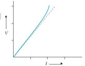
FIGURE 3.5 The dashed line represents the linear Ohm’s law. The solid line is the voltage V versus current I for a good conductor.
(b) The relation between V and I depends on the sign of V. In other words, if I is the current for a certain V, then reversing the direction of V keeping its magnitude fixed, does not produce a current of the same magnitude as I in the opposite direction (Fig. 3.6). This happens, for example, in a diode which we will study in Chapter 14.
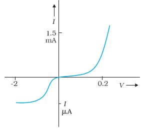
FIGURE 3.6 Characteristic curve of a diode. Note the different scales for negative and positive values of the voltage and current.
(c) The relation between V and I is not unique, i.e., there is more than one value of V for the same current I (Fig. 3.7). A material exhibiting such behaviour is GaAs.
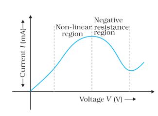
FIGURE 3.7 Variation of current versus voltage for GaAs.
Materials and devices not obeying Ohm’s law in the form of Eq. (3.3) are actually widely used in electronic circuits. In this and a few subsequent chapters, however, we will study the electrical currents in materials that obey Ohm’s law.
RESISTIVITY OF VARIOUS MATERIALS
The resistivities of various common materials are listed in Table 3.1. The materials are classified as conductors, semiconductors and insulators
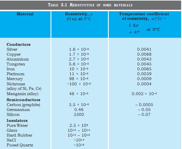
depending on their resistivities, in an increasing order of their values. Metals have low resistivities in the range of 10–8 \(% MathType!MTEF!2!1!+- % feaagKart1ev2aaatCvAUfeBSjuyZL2yd9gzLbvyNv2CaerbuLwBLn % hiov2DGi1BTfMBaeXatLxBI9gBaerbd9wDYLwzYbItLDharqqtubsr % 4rNCHbGeaGqiVu0Je9sqqrpepC0xbbL8F4rqqrFfpeea0xe9Lq-Jc9 % vqaqpepm0xbba9pwe9Q8fs0-yqaqpepae9pg0FirpepeKkFr0xfr-x % fr-xb9adbaqaaeGaciGaaiaabeqaamaabaabaaGcbaGaeyyQdCfaaa!3785! \Omega \)m to 10–6 \(% MathType!MTEF!2!1!+- % feaagKart1ev2aaatCvAUfeBSjuyZL2yd9gzLbvyNv2CaerbuLwBLn % hiov2DGi1BTfMBaeXatLxBI9gBaerbd9wDYLwzYbItLDharqqtubsr % 4rNCHbGeaGqiVu0Je9sqqrpepC0xbbL8F4rqqrFfpeea0xe9Lq-Jc9 % vqaqpepm0xbba9pwe9Q8fs0-yqaqpepae9pg0FirpepeKkFr0xfr-x % fr-xb9adbaqaaeGaciGaaiaabeqaamaabaabaaGcbaGaeyyQdCfaaa!3785! \Omega \)m. At the other end are insulators like ceramic, rubber and plastics having resistivities 1018 times greater than metals or more. In between the two are the semiconductors. These, however, have resistivities characteristically decreasing with a rise in temperature. The resistivities of semiconductors can be decreased by adding small amount of suitable impurities. This last feature is exploited in use of semiconductors for electronic devices.Commercially produced resistors for domestic use or in laboratories are of two major types: wire boubnd resistors and caron resistors. Wire bound resistors are made by winding the wires of an alloy, viz., manganin, constantan, nichrome or similar ones. The choice of these materials is dictated mostly by the fact that their resistivities are relatively insensitive to temperature. These resistances are typically in the range of a fraction of an ohm to a few hundred ohms.
Resistors in the higher range are made mostly from carbon. Carbon resistors are compact, inexpensive and thus find extensive use in electronic circuits. Carbon resistors are small in size and hence their values are given using a colour code.
The resistors have a set of co-axial coloured rings on them whose significance are listed in Table 3.2.
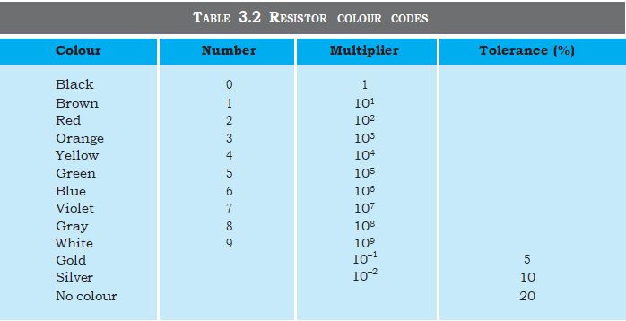
first two bands from the end indicate the first two significant figures of the resistance in ohms. The thirdband indicates the decimal multiplier (as listed in Table 3.2). The last band stands for tolerance or possible variation in percentage about the indicated values. Sometimes, this last band is absent and that indicates a tolerance of 20% (Fig.3.8).
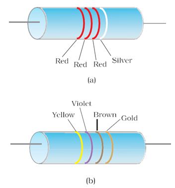
FIGURE 3.8 Colour coded resistors
(a) (22 × 102 \(% MathType!MTEF!2!1!+- % feaagKart1ev2aaatCvAUfeBSjuyZL2yd9gzLbvyNv2CaerbuLwBLn % hiov2DGi1BTfMBaeXatLxBI9gBaerbd9wDYLwzYbItLDharqqtubsr % 4rNCHbGeaGqiVu0Je9sqqrpepC0xbbL8F4rqqrFfpeea0xe9Lq-Jc9 % vqaqpepm0xbba9pwe9Q8fs0-yqaqpepae9pg0FirpepeKkFr0xfr-x % fr-xb9adbaqaaeGaciGaaiaabeqaamaabaabaaGcbaGaeyyQdCfaaa!3785! \Omega \)) ± 10%,
(b) (47 × 10 \(% MathType!MTEF!2!1!+- % feaagKart1ev2aaatCvAUfeBSjuyZL2yd9gzLbvyNv2CaerbuLwBLn % hiov2DGi1BTfMBaeXatLxBI9gBaerbd9wDYLwzYbItLDharqqtubsr % 4rNCHbGeaGqiVu0Je9sqqrpepC0xbbL8F4rqqrFfpeea0xe9Lq-Jc9 % vqaqpepm0xbba9pwe9Q8fs0-yqaqpepae9pg0FirpepeKkFr0xfr-x % fr-xb9adbaqaaeGaciGaaiaabeqaamaabaabaaGcbaGaeyyQdCfaaa!3785! \Omega \)) ± 5%.
For example, if the four colours are orange, blue, yellow and gold, the resistance value is 36 × 104 \(% MathType!MTEF!2!1!+- % feaagKart1ev2aaatCvAUfeBSjuyZL2yd9gzLbvyNv2CaerbuLwBLn % hiov2DGi1BTfMBaeXatLxBI9gBaerbd9wDYLwzYbItLDharqqtubsr % 4rNCHbGeaGqiVu0Je9sqqrpepC0xbbL8F4rqqrFfpeea0xe9Lq-Jc9 % vqaqpepm0xbba9pwe9Q8fs0-yqaqpepae9pg0FirpepeKkFr0xfr-x % fr-xb9adbaqaaeGaciGaaiaabeqaamaabaabaaGcbaGaeyyQdCfaaa!3785! \Omega \), with a tolerence value of 5%.
TEMPERATURE DEPENDENCE RESISTIVITY
\(% MathType!MTEF!2!1!+- % feaagKart1ev2aaatCvAUfeBSjuyZL2yd9gzLbvyNv2CaerbuLwBLn % hiov2DGi1BTfMBaeXatLxBI9gBaerbd9wDYLwzYbItLDharqqtubsr % 4rNCHbGeaGqiVu0Je9sqqrpepC0xbbL8F4rqqrFfpeea0xe9Lq-Jc9 % vqaqpepm0xbba9pwe9Q8fs0-yqaqpepae9pg0FirpepeKkFr0xfr-x % fr-xb9adbaqaaeGaciGaaiaabeqaamaabaabaaGcbaGaeqyWdi3aaS % baaSqaaiaadsfaaeqaaOGaeyypa0JaeqyWdi3aaSbaaSqaaiaaicda % aeqaaOWaamWaaeaacaaIXaGaey4kaSIaeqySde2aaeWaaeaacaWGub % GaeyOeI0IaamivamaaBaaaleaacaaIWaaabeaaaOGaayjkaiaawMca % aaGaay5waiaaw2faaaaa!46C1! {\rho _T} = {\rho _0}\left[ {1 + \alpha \left( {T - {T_0}} \right)} \right]\)(3.6)
where \(% MathType!MTEF!2!1!+- % feaagKart1ev2aaatCvAUfeBSjuyZL2yd9gzLbvyNv2CaerbuLwBLn % hiov2DGi1BTfMBaeXatLxBI9gBaerbd9wDYLwzYbItLDharqqtubsr % 4rNCHbGeaGqiVu0Je9sqqrpepC0xbbL8F4rqqrFfpeea0xe9Lq-Jc9 % vqaqpepm0xbba9pwe9Q8fs0-yqaqpepae9pg0FirpepeKkFr0xfr-x % fr-xb9adbaqaaeGaciGaaiaabeqaamaabaabaaGcbaGaeqyWdi3aaS % baaSqaaiaadsfaaeqaaaaa!38BB! {\rho _T}\) is the resistivity at a temperature T and\(% MathType!MTEF!2!1!+- % feaagKart1ev2aaatCvAUfeBSjuyZL2yd9gzLbvyNv2CaerbuLwBLn % hiov2DGi1BTfMBaeXatLxBI9gBaerbd9wDYLwzYbItLDharqqtubsr % 4rNCHbGeaGqiVu0Je9sqqrpepC0xbbL8F4rqqrFfpeea0xe9Lq-Jc9 % vqaqpepm0xbba9pwe9Q8fs0-yqaqpepae9pg0FirpepeKkFr0xfr-x % fr-xb9adbaqaaeGaciGaaiaabeqaamaabaabaaGcbaGaeqyWdi3aaS % baaSqaaiaadsfaaeqaaaaa!38BB! {\rho _0}\) is the same at a reference temperature T0. \(\alpha\) is called the temperature co-efficient of resistivity, and from Eq. (3.26), the dimension of \(\alpha\) is (Temperature)–1.
For metals, \(\alpha\) is positive and values of \(\alpha\) for some metals at T0 = 0°C are listed in Table 3.1.
The relation of Eq. (3.26) implies that a graph of \(% MathType!MTEF!2!1!+- % feaagKart1ev2aaatCvAUfeBSjuyZL2yd9gzLbvyNv2CaerbuLwBLn % hiov2DGi1BTfMBaeXatLxBI9gBaerbd9wDYLwzYbItLDharqqtubsr % 4rNCHbGeaGqiVu0Je9sqqrpepC0xbbL8F4rqqrFfpeea0xe9Lq-Jc9 % vqaqpepm0xbba9pwe9Q8fs0-yqaqpepae9pg0FirpepeKkFr0xfr-x % fr-xb9adbaqaaeGaciGaaiaabeqaamaabaabaaGcbaGaeqyWdi3aaS % baaSqaaiaadsfaaeqaaaaa!38BB! {\rho _T}\) plotted against T would be a straight line. At temperatures much lower than 0°C, the graph, however, deviates considerably from a straight line (Fig. 3.9).
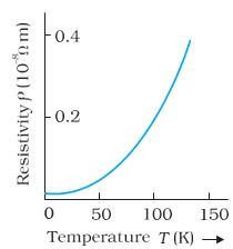
FIGURE 3.9
Resistivity \(% MathType!MTEF!2!1!+- % feaagKart1ev2aaatCvAUfeBSjuyZL2yd9gzLbvyNv2CaerbuLwBLn % hiov2DGi1BTfMBaeXatLxBI9gBaerbd9wDYLwzYbItLDharqqtubsr % 4rNCHbGeaGqiVu0Je9sqqrpepC0xbbL8F4rqqrFfpeea0xe9Lq-Jc9 % vqaqpepm0xbba9pwe9Q8fs0-yqaqpepae9pg0FirpepeKkFr0xfr-x % fr-xb9adbaqaaeGaciGaaiaabeqaamaabaabaaGcbaGaeqyWdi3aaS % baaSqaaiaadsfaaeqaaaaa!38BB! {\rho _T}\) of copper as a function of temperature T.
Equation (3.26) thus, can be used approximately over a limited range of T around any reference temperature T0, where the graph can be approximated as a straight line.
Some materials like Nichrome (which is an alloy of nickel, iron and chromium) exhibit a very weak dependence of resistivity with temperature (Fig. 3.10).
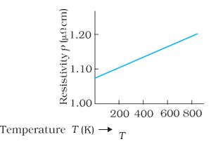
FIGURE 3.10 Resistivity \(% MathType!MTEF!2!1!+- % feaagKart1ev2aaatCvAUfeBSjuyZL2yd9gzLbvyNv2CaerbuLwBLn % hiov2DGi1BTfMBaeXatLxBI9gBaerbd9wDYLwzYbItLDharqqtubsr % 4rNCHbGeaGqiVu0Je9sqqrpepC0xbbL8F4rqqrFfpeea0xe9Lq-Jc9 % vqaqpepm0xbba9pwe9Q8fs0-yqaqpepae9pg0FirpepeKkFr0xfr-x % fr-xb9adbaqaaeGaciGaaiaabeqaamaabaabaaGcbaGaeqyWdi3aaS % baaSqaaiaadsfaaeqaaaaa!38BB! {\rho _T}\) of nichrome as a function of absolute temperature T.
Manganin and constantan have similar properties. These materials are thus widely used in wire bound standard resistors since their resistance values would change very little with temperatures.
Unlike metals, the resistivities of semiconductors decrease with increasing temperatures. A typical dependence is shown in Fig. 3.11.
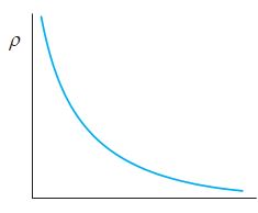
FIGURE 3.11. Temperature dependence of resistivity for a typical semiconductor.
We can qualitatively understand the temperature dependence of resistivity, in the light of our derivation of Eq. (3.23). From this equation, resistivity of a material is given by
\(% MathType!MTEF!2!1!+- % feaagKart1ev2aaatCvAUfeBSjuyZL2yd9gzLbvyNv2CaerbuLwBLn % hiov2DGi1BTfMBaeXatLxBI9gBaerbd9wDYLwzYbItLDharqqtubsr % 4rNCHbGeaGqiVu0Je9sqqrpepC0xbbL8F4rqqrFfpeea0xe9Lq-Jc9 % vqaqpepm0xbba9pwe9Q8fs0-yqaqpepae9pg0FirpepeKkFr0xfr-x % fr-xb9adbaqaaeGaciGaaiaabeqaamaabaabaaGcbaGaeqyWdiNaey % ypa0ZaaSaaaeaacaaIXaaabaGaeq4Wdmhaaiabg2da9maalaaabaGa % amyBaaqaaiaad6gacaWGLbWaaWbaaSqabeaacaaIYaaaaOGaeqiXdq % haaaaa!41E7! \rho = \frac{1}{\sigma } = \frac{m}{{n{e^2}\tau }}\)(3.27)
\(% MathType!MTEF!2!1!+- % feaagKart1ev2aaatCvAUfeBSjuyZL2yd9gzLbvyNv2CaerbuLwBLn % hiov2DGi1BTfMBaeXatLxBI9gBaerbd9wDYLwzYbItLDharqqtubsr % 4rNCHbGeaGqiVu0Je9sqqrpepC0xbbL8F4rqqrFfpeea0xe9Lq-Jc9 % vqaqpepm0xbba9pwe9Q8fs0-yqaqpepae9pg0FirpepeKkFr0xfr-x % fr-xb9adbaqaaeGaciGaaiaabeqaamaabaabaaGcbaGaeqyWdihaaa!37B6! \rho \) thus depends inversely both on the number n of free electrons per unit volume and on the average time \(% MathType!MTEF!2!1!+- % feaagKart1ev2aaatCvAUfeBSjuyZL2yd9gzLbvyNv2CaerbuLwBLn % hiov2DGi1BTfMBaeXatLxBI9gBaerbd9wDYLwzYbItLDharqqtubsr % 4rNCHbGeaGqiVu0Je9sqqrpepC0xbbL8F4rqqrFfpeea0xe9Lq-Jc9 % vqaqpepm0xbba9pwe9Q8fs0-yqaqpepae9pg0FirpepeKkFr0xfr-x % fr-xb9adbaqaaeGaciGaaiaabeqaamaabaabaaGcbaGaeqiXdqhaaa!37BB! \tau \) between collisions. As we increase temperature, average speed of the electrons, which act as the carriers of current, increases resulting in more frequent collisions. The average time of collisions \(% MathType!MTEF!2!1!+- % feaagKart1ev2aaatCvAUfeBSjuyZL2yd9gzLbvyNv2CaerbuLwBLn % hiov2DGi1BTfMBaeXatLxBI9gBaerbd9wDYLwzYbItLDharqqtubsr % 4rNCHbGeaGqiVu0Je9sqqrpepC0xbbL8F4rqqrFfpeea0xe9Lq-Jc9 % vqaqpepm0xbba9pwe9Q8fs0-yqaqpepae9pg0FirpepeKkFr0xfr-x % fr-xb9adbaqaaeGaciGaaiaabeqaamaabaabaaGcbaGaeqiXdqhaaa!37BB! \tau \), thus decreases with temperature.
In a metal, n is not dependent on temperature to any appreciable extent and thus the decrease in the value of \(% MathType!MTEF!2!1!+- % feaagKart1ev2aaatCvAUfeBSjuyZL2yd9gzLbvyNv2CaerbuLwBLn % hiov2DGi1BTfMBaeXatLxBI9gBaerbd9wDYLwzYbItLDharqqtubsr % 4rNCHbGeaGqiVu0Je9sqqrpepC0xbbL8F4rqqrFfpeea0xe9Lq-Jc9 % vqaqpepm0xbba9pwe9Q8fs0-yqaqpepae9pg0FirpepeKkFr0xfr-x % fr-xb9adbaqaaeGaciGaaiaabeqaamaabaabaaGcbaGaeqiXdqhaaa!37BB! \tau \) with rise in temperature causes \(% MathType!MTEF!2!1!+- % feaagKart1ev2aaatCvAUfeBSjuyZL2yd9gzLbvyNv2CaerbuLwBLn % hiov2DGi1BTfMBaeXatLxBI9gBaerbd9wDYLwzYbItLDharqqtubsr % 4rNCHbGeaGqiVu0Je9sqqrpepC0xbbL8F4rqqrFfpeea0xe9Lq-Jc9 % vqaqpepm0xbba9pwe9Q8fs0-yqaqpepae9pg0FirpepeKkFr0xfr-x % fr-xb9adbaqaaeGaciGaaiaabeqaamaabaabaaGcbaGaeqyWdihaaa!37B6! \rho \) to increase as we have observed.
For insulators and semiconductors, however, n increases with temperature. This increase more than compensates any decrease in \(% MathType!MTEF!2!1!+- % feaagKart1ev2aaatCvAUfeBSjuyZL2yd9gzLbvyNv2CaerbuLwBLn % hiov2DGi1BTfMBaeXatLxBI9gBaerbd9wDYLwzYbItLDharqqtubsr % 4rNCHbGeaGqiVu0Je9sqqrpepC0xbbL8F4rqqrFfpeea0xe9Lq-Jc9 % vqaqpepm0xbba9pwe9Q8fs0-yqaqpepae9pg0FirpepeKkFr0xfr-x % fr-xb9adbaqaaeGaciGaaiaabeqaamaabaabaaGcbaGaeqiXdqhaaa!37BB! \tau \) in Eq.(3.23) so that for such materials, \(% MathType!MTEF!2!1!+- % feaagKart1ev2aaatCvAUfeBSjuyZL2yd9gzLbvyNv2CaerbuLwBLn % hiov2DGi1BTfMBaeXatLxBI9gBaerbd9wDYLwzYbItLDharqqtubsr % 4rNCHbGeaGqiVu0Je9sqqrpepC0xbbL8F4rqqrFfpeea0xe9Lq-Jc9 % vqaqpepm0xbba9pwe9Q8fs0-yqaqpepae9pg0FirpepeKkFr0xfr-x % fr-xb9adbaqaaeGaciGaaiaabeqaamaabaabaaGcbaGaeqyWdihaaa!37B6! \rho \) decreases with temperature.
EXAMPLE 3
An electric toaster uses nichrome for its heating element. When a negligibly small current passes through it, its resistance at room temperature (27.0 °C) is found to be 75.3\(% MathType!MTEF!2!1!+- % feaagKart1ev2aaatCvAUfeBSjuyZL2yd9gzLbvyNv2CaerbuLwBLn % hiov2DGi1BTfMBaeXatLxBI9gBaerbd9wDYLwzYbItLDharqqtubsr % 4rNCHbGeaGqiVu0Je9sqqrpepC0xbbL8F4rqqrFfpeea0xe9Lq-Jc9 % vqaqpepm0xbba9pwe9Q8fs0-yqaqpepae9pg0FirpepeKkFr0xfr-x % fr-xb9adbaqaaeGaciGaaiaabeqaamaabaabaaGcbaGaeyyQdCfaaa!3785! \Omega \). When the toaster is connected to a 230 V supply, the current settles, after a few seconds, to a steady value of 2.68 A. What is the steady temperature of the nichrome element? The temperature coefficient of resistance of nichrome averaged over the temperature range involved, is 1.70 × 10⁻⁴ °C–1.
SOLUTION
When the current through the element is very small, heating effects can be ignored and the temperature T1 of the element is the same as room temperature. When the toaster is connected to the supply, its initial current will be slightly higher than its steady value of 2.68 A. But due to heating effect of the current, the temperature will rise. This will cause an increase in resistance and a slight decrease in current. In a few seconds, a steady state will be reached when temperature will rise no further, and both the resistance of the element and the current drawn will achieve steady values. The resistance R2 at the steady temperature T2 is
\(% MathType!MTEF!2!1!+- % feaagKart1ev2aaatCvAUfeBSjuyZL2yd9gzLbvyNv2CaerbuLwBLn % hiov2DGi1BTfMBaeXatLxBI9gBaerbd9wDYLwzYbItLDharqqtubsr % 4rNCHbGeaGqiVu0Je9sqqrpepC0xbbL8F4rqqrFfpeea0xe9Lq-Jc9 % vqaqpepm0xbba9pwe9Q8fs0-yqaqpepae9pg0FirpepeKkFr0xfr-x % fr-xb9adbaqaaeGaciGaaiaabeqaamaabaabaaGcbaGaeqyWdiNaey % ypa0ZaaSaaaeaacaaIXaaabaGaeq4Wdmhaaiabg2da9maalaaabaGa % amyBaaqaaiaad6gacaWGLbWaaWbaaSqabeaacaaIYaaaaOGaeqiXdq % haaaaa!41E7! \rho = \frac{1}{\sigma } = \frac{m}{{n{e^2}\tau }}\)(3.27)
Using the relation
\(% MathType!MTEF!2!1!+- % feaagKart1ev2aaatCvAUfeBSjuyZL2yd9gzLbvyNv2CaerbuLwBLn % hiov2DGi1BTfMBaeXatLxBI9gBaerbd9wDYLwzYbItLDharqqtubsr % 4rNCHbGeaGqiVu0Je9sqqrpepC0xbbL8F4rqqrFfpeea0xe9Lq-Jc9 % vqaqpepm0xbba9pwe9Q8fs0-yqaqpepae9pg0FirpepeKkFr0xfr-x % fr-xb9adbaqaaeGaciGaaiaabeqaamaabaabaaGcbaGaamOuamaaBa % aaleaacaaIYaaabeaakiabg2da9iaadkfadaWgaaWcbaGaaGymaaqa % baGcdaWadaqaaiaaigdacqGHRaWkcqaHXoqydaqadaqaaiaadsfada % WgaaWcbaGaaGOmaaqabaGccqGHsislcaWGubWaaSbaaSqaaiaaigda % aeqaaaGccaGLOaGaayzkaaaacaGLBbGaayzxaaaaaa!45C6! {R_2} = {R_1}\left[ {1 + \alpha \left( {{T_2} - {T_1}} \right)} \right]\)
with \(\alpha\) = 1.70 × 10⁻⁴ °C–1, we get
\(% MathType!MTEF!2!1!+- % feaagKart1ev2aaatCvAUfeBSjuyZL2yd9gzLbvyNv2CaerbuLwBLn % hiov2DGi1BTfMBaeXatLxBI9gBaerbd9wDYLwzYbItLDharqqtubsr % 4rNCHbGeaGqiVu0Je9sqqrpepC0xbbL8F4rqqrFfpeea0xe9Lq-Jc9 % vqaqpepm0xbba9pwe9Q8fs0-yqaqpepae9pg0FirpepeKkFr0xfr-x % fr-xb9adbaqaaeGaciGaaiaabeqaamaabaabaaGcbaGaamivamaaBa % aaleaacaaIYaaabeaakiabgkHiTiaadsfadaWgaaWcbaGaaGymaaqa % baGccqGH9aqpdaWcaaqaamaabmaabaGaaGioaiaaiwdacaGGUaGaaG % ioaiabgkHiTiaaiEdacaaI1aGaaiOlaiaaiodaaiaawIcacaGLPaaa % aeaadaqadaqaaiaaiEdacaaI1aGaaiOlaiaaiodaaiaawIcacaGLPa % aacqGHxdaTcaaIXaGaaiOlaiaaiEdacaaIWaGaey41aqRaaGymaiaa % icdadaahaaWcbeqaaiabgkHiTiaaisdaaaaaaOGaeyypa0JaaGioai % aaikdacaaIWaWaaWbaaSqabeaacqWIyiYBaaGccaWGdbaaaa!5844! {T_2} - {T_1} = \frac{{\left( {85.8 - 75.3} \right)}}{{\left( {75.3} \right) \times 1.70 \times {{10}^{ - 4}}}} = {820^ \circ }C\)
that is, T2 = (820 + 27.0) °C = 847 °C
Thus, the steady temperature of the heating element (when heating effect due to the current equals heat loss to the surroundings) is 847 °C.
EXAMPLE 4
The resistance of the platinum wire of a platinum resistance thermometer at the ice point is 5\(% MathType!MTEF!2!1!+- % feaagKart1ev2aaatCvAUfeBSjuyZL2yd9gzLbvyNv2CaerbuLwBLn % hiov2DGi1BTfMBaeXatLxBI9gBaerbd9wDYLwzYbItLDharqqtubsr % 4rNCHbGeaGqiVu0Je9sqqrpepC0xbbL8F4rqqrFfpeea0xe9Lq-Jc9 % vqaqpepm0xbba9pwe9Q8fs0-yqaqpepae9pg0FirpepeKkFr0xfr-x % fr-xb9adbaqaaeGaciGaaiaabeqaamaabaabaaGcbaGaeyyQdCfaaa!3785! \Omega \) and at steam point is 5.23\(% MathType!MTEF!2!1!+- % feaagKart1ev2aaatCvAUfeBSjuyZL2yd9gzLbvyNv2CaerbuLwBLn % hiov2DGi1BTfMBaeXatLxBI9gBaerbd9wDYLwzYbItLDharqqtubsr % 4rNCHbGeaGqiVu0Je9sqqrpepC0xbbL8F4rqqrFfpeea0xe9Lq-Jc9 % vqaqpepm0xbba9pwe9Q8fs0-yqaqpepae9pg0FirpepeKkFr0xfr-x % fr-xb9adbaqaaeGaciGaaiaabeqaamaabaabaaGcbaGaeyyQdCfaaa!3785! \Omega \). When the thermometer is inserted in a hot bath, the resistance of the platinum wire is 5.795 \(% MathType!MTEF!2!1!+- % feaagKart1ev2aaatCvAUfeBSjuyZL2yd9gzLbvyNv2CaerbuLwBLn % hiov2DGi1BTfMBaeXatLxBI9gBaerbd9wDYLwzYbItLDharqqtubsr % 4rNCHbGeaGqiVu0Je9sqqrpepC0xbbL8F4rqqrFfpeea0xe9Lq-Jc9 % vqaqpepm0xbba9pwe9Q8fs0-yqaqpepae9pg0FirpepeKkFr0xfr-x % fr-xb9adbaqaaeGaciGaaiaabeqaamaabaabaaGcbaGaeyyQdCfaaa!3785! \Omega \). Calculate the temperature of the bath.
SOLUTION
R0 = 5 \(% MathType!MTEF!2!1!+- % feaagKart1ev2aaatCvAUfeBSjuyZL2yd9gzLbvyNv2CaerbuLwBLn % hiov2DGi1BTfMBaeXatLxBI9gBaerbd9wDYLwzYbItLDharqqtubsr % 4rNCHbGeaGqiVu0Je9sqqrpepC0xbbL8F4rqqrFfpeea0xe9Lq-Jc9 % vqaqpepm0xbba9pwe9Q8fs0-yqaqpepae9pg0FirpepeKkFr0xfr-x % fr-xb9adbaqaaeGaciGaaiaabeqaamaabaabaaGcbaGaeyyQdCfaaa!3785! \Omega \), R100 = 5.23\(% MathType!MTEF!2!1!+- % feaagKart1ev2aaatCvAUfeBSjuyZL2yd9gzLbvyNv2CaerbuLwBLn % hiov2DGi1BTfMBaeXatLxBI9gBaerbd9wDYLwzYbItLDharqqtubsr % 4rNCHbGeaGqiVu0Je9sqqrpepC0xbbL8F4rqqrFfpeea0xe9Lq-Jc9 % vqaqpepm0xbba9pwe9Q8fs0-yqaqpepae9pg0FirpepeKkFr0xfr-x % fr-xb9adbaqaaeGaciGaaiaabeqaamaabaabaaGcbaGaeyyQdCfaaa!3785! \Omega \) and Rt = 5.795 \(% MathType!MTEF!2!1!+- % feaagKart1ev2aaatCvAUfeBSjuyZL2yd9gzLbvyNv2CaerbuLwBLn % hiov2DGi1BTfMBaeXatLxBI9gBaerbd9wDYLwzYbItLDharqqtubsr % 4rNCHbGeaGqiVu0Je9sqqrpepC0xbbL8F4rqqrFfpeea0xe9Lq-Jc9 % vqaqpepm0xbba9pwe9Q8fs0-yqaqpepae9pg0FirpepeKkFr0xfr-x % fr-xb9adbaqaaeGaciGaaiaabeqaamaabaabaaGcbaGaeyyQdCfaaa!3785! \Omega \)
\(% MathType!MTEF!2!1!+- % feaagKart1ev2aaatCvAUfeBSjuyZL2yd9gzLbvyNv2CaerbuLwBLn % hiov2DGi1BTfMBaeXatLxBI9gBaerbd9wDYLwzYbItLDharqqtubsr % 4rNCHbGeaGqiVu0Je9sqqrpepC0xbbL8F4rqqrFfpeea0xe9Lq-Jc9 % vqaqpepm0xbba9pwe9Q8fs0-yqaqpepae9pg0FirpepeKkFr0xfr-x % fr-xb9adbaqaaeGaciGaaiaabeqaamaabaabaaGceaqabeaacaWGob % Gaam4BaiaadEhacaGGSaGaaGPaVlaaykW7caaMc8UaamiDaiabg2da % 9maalaaabaGaamOuamaaBaaaleaacaWG0baabeaakiabgkHiTiaadk % fadaWgaaWcbaGaaGimaaqabaaakeaacaWGsbWaaSbaaSqaaiaaigda % caaIWaGaaGimaaqabaGccqGHsislcaWGsbWaaSbaaSqaaiaaicdaae % qaaaaakiabgEna0kaaigdacaaIWaGaaGimaiaacYcacaaMc8UaaGPa % VlaadkfadaWgaaWcbaGaamiDaaqabaGccqGH9aqpcaWGsbWaaSbaaS % qaaiaaicdaaeqaaOWaaeWaaeaacaaIXaGaey4kaSIaeqySdeMaamiD % aaGaayjkaiaawMcaaaqaaiaaykW7caaMc8UaaGPaVlaaykW7caaMc8 % UaaGPaVlaaykW7caaMc8UaaGPaVlaaykW7caaMc8UaaGPaVlaaykW7 % caaMc8UaaGPaVlaaykW7caaMc8Uaeyypa0ZaaSaaaeaacaaI1aGaai % OlaiaaiEdacaaI5aGaaGynaiabgkHiTiaaiwdaaeaacaaI1aGaaiOl % aiaaikdacaaIZaGaeyOeI0IaaGynaaaacqGHxdaTcaaIXaGaaGimai % aaicdaaeaacaaMc8UaaGPaVlaaykW7caaMc8UaaGPaVlaaykW7caaM % c8UaaGPaVlaaykW7caaMc8UaaGPaVlaaykW7caaMc8UaaGPaVlaayk % W7caaMc8UaaGPaVlabg2da9maalaaabaGaaGimaiaac6cacaaI3aGa % aGyoaiaaiwdaaeaacaaIWaGaaiOlaiaaikdacaaIZaaaaiabgEna0k % aaigdacaaIWaGaaGimaiabg2da9iaaiodacaaI0aGaaGynaiaac6ca % caaI2aGaaG4namaaCaaaleqabaGaeSigI8gaaOGaam4yaaaaaa!B4EC! \begin{array}{l} Now,\,\,\,t = \frac{{{R_t} - {R_0}}}{{{R_{100}} - {R_0}}} \times 100,\,\,{R_t} = {R_0}\left( {1 + \alpha t} \right)\\ \,\,\,\,\,\,\,\,\,\,\,\,\,\,\,\,\, = \frac{{5.795 - 5}}{{5.23 - 5}} \times 100\\ \,\,\,\,\,\,\,\,\,\,\,\,\,\,\,\,\, = \frac{{0.795}}{{0.23}} \times 100 = {345.67^ \circ }c \end{array}\)
ELECTRICAL ENERGY, POWER
Consider a conductor with end points A and B, in which a current I is flowing from A to B. The electric potential at A and B are denoted by V (A) and V (B) respectively. Since current is flowing from A to B, V (A) > V (B) and the potential difference across AB is V = V(A) – V(B) > 0.
In a time interval \(\Delta\)t, an amount of charge \(\Delta\)Q = I \(\Delta\)t travels from A to B. The potential energy of the charge at A, by definition, was Q V (A) and similarly at B, it is Q V(B). Thus, change in its potential energy \(\Delta\)Upotis
\(\Delta\)Upot = Final potential energy – Initial potential energy
= \(\Delta\)Q[(V (B) – V (A)] = –\(\Delta\)Q V
= –I V\(\Delta\)t < 0 (3.28)
If charges moved without collisions through the conductor, their kinetic energy would also change so that the total energy is unchanged. Conservation of total energy would then imply that
\(% MathType!MTEF!2!1!+- % feaagKart1ev2aaatCvAUfeBSjuyZL2yd9gzLbvyNv2CaerbuLwBLn % hiov2DGi1BTfMBaeXatLxBI9gBaerbd9wDYLwzYbItLDharqqtubsr % 4rNCHbGeaGqiVu0Je9sqqrpepC0xbbL8F4rqqrFfpeea0xe9Lq-Jc9 % vqaqpepm0xbba9pwe9Q8fs0-yqaqpepae9pg0FirpepeKkFr0xfr-x % fr-xb9adbaqaaeGaciGaaiaabeqaamaabaabaaGcbaGaeyiLdqKaam % 4saiabg2da9iabgkHiTiabgs5aejaadwfadaWgaaWcbaGaamiCaiaa % d+gacaWG0baabeaaaaa!3F6F! \Delta K = - \Delta {U_{pot}}\) (3.29)
that is,
\(% MathType!MTEF!2!1!+- % feaagKart1ev2aaatCvAUfeBSjuyZL2yd9gzLbvyNv2CaerbuLwBLn % hiov2DGi1BTfMBaeXatLxBI9gBaerbd9wDYLwzYbItLDharqqtubsr % 4rNCHbGeaGqiVu0Je9sqqrpepC0xbbL8F4rqqrFfpeea0xe9Lq-Jc9 % vqaqpepm0xbba9pwe9Q8fs0-yqaqpepae9pg0FirpepeKkFr0xfr-x % fr-xb9adbaqaaeGaciGaaiaabeqaamaabaabaaGcbaGaeyiLdqKaam % 4saiabg2da9iaadMeacaWGwbGaeyiLdqKaamiDaiabg6da+iaaicda % aaa!3EFE! \Delta K = IV\Delta t > 0\) (3.30)
Thus, in case charges were moving freely through the conductor under the action of electric field, their kinetic energy would increase as they move. We have, however, seen earlier that on the average, charge carriers do not move with acceleration but with a steady drift velocity. This is because of the collisions with ions and atoms during transit. During collisions, the energy gained by the charges thus is shared with the atoms. The atoms vibrate more vigorously, i.e., the conductor heats up. Thus, in an actual conductor, an amount of energy dissipated as heat in the conductor during the time interval \(\Delta\)t is,
\(\Delta\)W = I V\(\Delta\)t (3.31)
The energy dissipated per unit time is the power dissipated
P = \(\Delta\)W/\(\Delta\)t and we have,
P = I V (3.32)
Using Ohm’s law V = IR, we get
P = I 2 R = V 2/R (3.33)
as the power loss (“ohmic loss”) in a conductor of resistance R carrying a current I. It is this power which heats up, for example, the coil of an electric bulb to incandescence, radiating out heat and light.
Where does the power come from? As we have
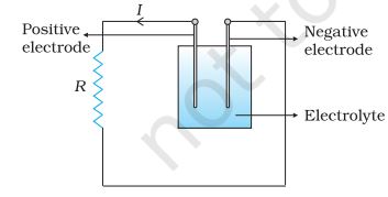
FIGURE 3.12 Heat is produced in the resistor R which is connected across the terminals of a cell. The energy dissipated in the resistor R comes from the chemical energy of the electrolyte.
The expressions for power, Eqs. (3.32) and (3.33), show the dependence of the power dissipated in a resistor R on the current through it and the voltage across it.
Equation (3.33) has an important application to power transmission. Electrical power is transmitted from power stations to homes and factories, which may be hundreds of miles away, via transmission cables. One obviously wants to minimise the power loss in the transmission cables connecting the power stations to homes and factories. We shall see now how this can be achieved. Consider a device R, to which a power P is to be delivered via transmission cables having a resistance Rc to be dissipated by it finally.
If V is the voltage across R and I the current through it, then
P = V I (3.34)
The connecting wires from the power station to the device has a finite resistance Rc. The power dissipated in the connecting wires, which is wasted is Pc with
\(% MathType!MTEF!2!1!+- % feaagKart1ev2aaatCvAUfeBSjuyZL2yd9gzLbvyNv2CaerbuLwBLn % hiov2DGi1BTfMBaeXatLxBI9gBaerbd9wDYLwzYbItLDharqqtubsr % 4rNCHbGeaGqiVu0Je9sqqrpepC0xbbL8F4rqqrFfpeea0xe9Lq-Jc9 % vqaqpepm0xbba9pwe9Q8fs0-yqaqpepae9pg0FirpepeKkFr0xfr-x % fr-xb9adbaqaaeGaciGaaiaabeqaamaabaabaaGceaqabeaacaWGqb % WaaSbaaSqaaiaadogaaeqaaOGaeyypa0JaamysamaaCaaaleqabaGa % aGOmaaaakiaadkfadaWgaaWcbaGaam4yaaqabaaakeaacqGH9aqpda % WcaaqaaiaadcfadaahaaWcbeqaaiaaikdaaaGccaWGsbWaaSbaaSqa % aiaadogaaeqaaaGcbaGaamOvamaaCaaaleqabaGaaGOmaaaaaaGcca % aMc8UaaGPaVlaaykW7caaMc8UaaGPaVlaaykW7caaMc8UaaGPaVlaa % ykW7caaMc8UaaGPaVlaaykW7caaMc8UaaGPaVlaaykW7caaMc8UaaG % PaVlaaykW7caaMc8UaaGPaVpaabmaabaGaaG4maiaac6cacaaIZaGa % aGynaaGaayjkaiaawMcaaaaaaa!669D! \begin{array}{l} {P_c} = {I^2}{R_c}\\ = \frac{{{P^2}{R_c}}}{{{V^2}}}\,\,\,\,\,\,\,\,\,\,\,\,\,\,\,\,\,\,\,\,\left( {3.35} \right) \end{array}\)
from Eq. (3.32). Thus, to drive a device of power P, the power wasted in the connecting wires is inversely proportional to V 2. The transmission cables from power stations are hundreds of miles long and their resistance Rc is considerable. To reduce Pc, these wires carry current at enormous values of V and this is the reason for the high voltage danger signs on transmission lines — a common sight as we move away from populated areas. Using electricity at such voltages is not safe and hence at the other end, a device called a transformer lowers the voltage to a value suitable for use.
COMBINATION OF RESISTORS – SERIES AND PARALLEL
The current through a single resistor R across which there is a potential difference V is given by Ohm’s law I = V/R. Resistors are sometimes joined together and there are simple rules for calculation of equivalent resistance of such combination.
Two resistors are said to be in series if only one of their end points is joined (Fig. 3.13).

FIGURE 3.13 A series combination of two resistors R1 and R2.
If a third resistor is joined with the series combination of the two (Fig. 3.14), then all three are said to be in series. Clearly, we can extend this definition to series combination of any number of resistors.

FIGURE 3.14 A series combination of three resistors R1, R2, R3.
Two or more resistors are said to be in parallel if one end of all the resistors is joined together and similarly the other ends joined together (Fig. 3.15).
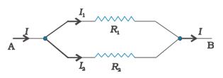
FIGURE 3.15 Two resistors R1 and R2 connected in parallel.
Consider two resistors R1 and R2 in series. The charge which leaves R1 must be entering R2. Since current measures the rate of flow of charge, this means that the same current I flows through R1 and R2. By Ohm’s law:
Potential difference across R1 = V1 = I R1, and Potential difference across R2 = V2 = I R2.
The potential difference V across the combination is V1+V2. Hence,
V = V1+ V2 = I (R1 + R2) (3.36)
This is as if the combination had an equivalent resistance Req, which by Ohm’s law is
\(% MathType!MTEF!2!1!+- % feaagKart1ev2aaatCvAUfeBSjuyZL2yd9gzLbvyNv2CaerbuLwBLn % hiov2DGi1BTfMBaeXatLxBI9gBaerbd9wDYLwzYbItLDharqqtubsr % 4rNCHbGeaGqiVu0Je9sqqrpepC0xbbL8F4rqqrFfpeea0xe9Lq-Jc9 % vqaqpepm0xbba9pwe9Q8fs0-yqaqpepae9pg0FirpepeKkFr0xfr-x % fr-xb9adbaqaaeGaciGaaiaabeqaamaabaabaaGcbaGaamOuamaaBa % aaleaacaWGLbGaamyCaaqabaGccqGHHjIUdaWcaaqaaiaadAfaaeaa % caWGjbaaaiabg2da9maabmaabaGaamOuamaaBaaaleaacaaIXaaabe % aakiabgUcaRiaadkfadaWgaaWcbaGaaGOmaaqabaaakiaawIcacaGL % Paaaaaa!4367! {R_{eq}} \equiv \frac{V}{I} = \left( {{R_1} + {R_2}} \right)\) (3.37)
If we had three resistors connected in series, then similarly
V = I R1 + I R2 + I R3 = I (R1+ R2+ R3). (3.38)
This obviously can be extended to a series combination of any number n of resistors R1, R2 , Rn. The equivalent resistance Req is
Req = R1 + R2 + . . . + Rn (3.39)
Consider now the parallel combination of two resistors (Fig. 3.15). The charge that flows in at A from the left flows out partly through R1 and partly through R2. The currents I, I1, I2 shown in the figure are the rates of flow of charge at the points indicated. Hence,
I = I1 + I2 (3.40)
The potential difference between A and B is given by the Ohm’s law applied to R1
V = I1 R1 (3.41)
Also, Ohm’s law applied to R2 gives
V = I2 R2 (3.42)
\(% MathType!MTEF!2!1!+- % feaagKart1ev2aaatCvAUfeBSjuyZL2yd9gzLbvyNv2CaerbuLwBLn % hiov2DGi1BTfMBaeXatLxBI9gBaerbd9wDYLwzYbItLDharqqtubsr % 4rNCHbGeaGqiVu0Je9sqqrpepC0xbbL8F4rqqrFfpeea0xe9Lq-Jc9 % vqaqpepm0xbba9pwe9Q8fs0-yqaqpepae9pg0FirpepeKkFr0xfr-x % fr-xb9adbaqaaeGaciGaaiaabeqaamaabaabaaGcbaGaeyinIWLaam % ysaiabg2da9iaadMeadaWgaaWcbaGaaGymaaqabaGccqGHRaWkcaWG % jbWaaSbaaSqaaiaaigdaaeqaaOGaeyypa0ZaaSaaaeaacaWGwbaaba % GaamOuamaaBaaaleaacaaIXaaabeaaaaGccqGHRaWkdaWcaaqaaiaa % dAfaaeaacaWGsbWaaSbaaSqaaiaaikdaaeqaaaaakiabg2da9iaadA % fadaqadaqaamaalaaabaGaaGymaaqaaiaadkfadaWgaaWcbaGaaGym % aaqabaaaaOGaey4kaSYaaSaaaeaacaaIXaaabaGaamOuamaaBaaale % aacaaIYaaabeaaaaaakiaawIcacaGLPaaaaaa!4E2A! \therefore I = {I_1} + {I_1} = \frac{V}{{{R_1}}} + \frac{V}{{{R_2}}} = V\left( {\frac{1}{{{R_1}}} + \frac{1}{{{R_2}}}} \right)\) (3.43)
If the combination was replaced by an equivalent resistance Req, we would have, by Ohm’s law
\(% MathType!MTEF!2!1!+- % feaagKart1ev2aaatCvAUfeBSjuyZL2yd9gzLbvyNv2CaerbuLwBLn % hiov2DGi1BTfMBaeXatLxBI9gBaerbd9wDYLwzYbItLDharqqtubsr % 4rNCHbGeaGqiVu0Je9sqqrpepC0xbbL8F4rqqrFfpeea0xe9Lq-Jc9 % vqaqpepm0xbba9pwe9Q8fs0-yqaqpepae9pg0FirpepeKkFr0xfr-x % fr-xb9adbaqaaeGaciGaaiaabeqaamaabaabaaGcbaGaamysaiabg2 % da9maalaaabaGaamOvaaqaaiaadkfadaWgaaWcbaGaamyzaiaadgha % aeqaaaaaaaa!3B98! I = \frac{V}{{{R_{eq}}}}\) (3.44)
Hence,
\(% MathType!MTEF!2!1!+- % feaagKart1ev2aaatCvAUfeBSjuyZL2yd9gzLbvyNv2CaerbuLwBLn % hiov2DGi1BTfMBaeXatLxBI9gBaerbd9wDYLwzYbItLDharqqtubsr % 4rNCHbGeaGqiVu0Je9sqqrpepC0xbbL8F4rqqrFfpeea0xe9Lq-Jc9 % vqaqpepm0xbba9pwe9Q8fs0-yqaqpepae9pg0FirpepeKkFr0xfr-x % fr-xb9adbaqaaeGaciGaaiaabeqaamaabaabaaGcbaWaaSaaaeaaca % aIXaaabaGaamOuamaaBaaaleaacaWGLbGaamyCaaqabaaaaOGaeyOe % I0YaaSaaaeaacaaIXaaabaGaamOuamaaBaaaleaacaaIXaaabeaaaa % GccaGGSaWaaSaaaeaacaaIXaaabaGaamOuamaaBaaaleaacaaIYaaa % beaaaaaaaa!4068! \frac{1}{{{R_{eq}}}} - \frac{1}{{{R_1}}},\frac{1}{{{R_2}}}\) (3.45)
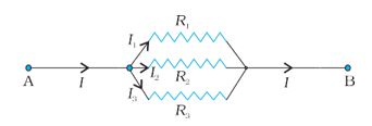
FIGURE 3.16 Parallel combination of three resistors R1, R2 and R3.
It should be noted that because of the symmetry of the network, the great power of Kirchhoff’s rules has not been very apparent in Example 3.6. In a general network, there will be no such simplification due to symmetry, and only by application of Kirchhoff’s rules to junctions and closed loops (as many as necessary to solve the unknowns in the network) can we handle the problem. This will be illustrated in Example 3.7.
EXAMPLE 7
Determine the current in each branch of the network shown in Fig. 3.24.
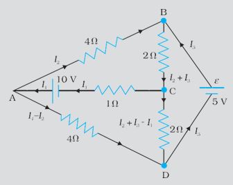
Fig. 3.24.
SOLUTION
Each branch of the network is assigned an unknown current to be determined by the application of Kirchhoff’s rules. To reduce the number of unknowns at the outset, the first rule of Kirchhoff is used at every junction to assign the unknown current in each branch. We then have three unknowns I1, I2 and I3 which can be found by applying the second rule of Kirchhoff to three different closed loops.
Kirchhoff’s second rule for the closed loop ADCA gives,
10 – 4(I1– I2) + 2(I2 + I3 – I1) – I1 = 0 [3.80(a)]
that is, 7I1– 6I2 – 2I3 = 10
For the closed loop ABCA, we get
10 – 4I2– 2 (I2 + I3) – I1 = 0
that is, I1 + 6I2 + 2I3 =10 [3.80(b)]
For the closed loop BCDEB, we get
5 – 2 (I2 + I3 ) – 2 (I2 + I3 – I1) = 0
that is, 2I1 – 4I2 – 4I3 = –5 [3.80(c)]
Equations (3.80 a, b, c) are three simultaneous equations in three unknowns. These can be solved by the usual method to give
\(% MathType!MTEF!2!1!+- % feaagKart1ev2aaatCvAUfeBSjuyZL2yd9gzLbvyNv2CaerbuLwBLn % hiov2DGi1BTfMBaeXatLxBI9gBaerbd9wDYLwzYbItLDharqqtubsr % 4rNCHbGeaGqiVu0Je9sqqrpepC0xbbL8F4rqqrFfpeea0xe9Lq-Jc9 % vqaqpepm0xbba9pwe9Q8fs0-yqaqpepae9pg0FirpepeKkFr0xfr-x % fr-xb9adbaqaaeGaciGaaiaabeqaamaabaabaaGcbaGaamysamaaBa % aaleaacaaIXaaabeaakiabg2da9iaaikdacaGGUaGaaGynaiaadgea % caGGSaGaamysamaaBaaaleaacaaIYaaabeaakiabg2da9maalaaaba % GaaGynaaqaaiaaiIdaaaGaamyqaiaacYcacaWGjbWaaSbaaSqaaiaa % iodaaeqaaOGaeyypa0JaaGymamaalaaabaGaaG4naaqaaiaaiIdaaa % Gaamyqaaaa!4806! {I_1} = 2.5A,{I_2} = \frac{5}{8}A,{I_3} = 1\frac{7}{8}A\)
The currents in the various branches of the network are
\(% MathType!MTEF!2!1!+- % feaagKart1ev2aaatCvAUfeBSjuyZL2yd9gzLbvyNv2CaerbuLwBLn % hiov2DGi1BTfMBaeXatLxBI9gBaerbd9wDYLwzYbItLDharqqtubsr % 4rNCHbGeaGqiVu0Je9sqqrpepC0xbbL8F4rqqrFfpeea0xe9Lq-Jc9 % vqaqpepm0xbba9pwe9Q8fs0-yqaqpepae9pg0FirpepeKkFr0xfr-x % fr-xb9adbaqaaeGaciGaaiaabeqaamaabaabaaGceaqabeaacaWGbb % GaamOqaiaacQdadaWcaaqaaiaaiwdaaeaacaaI4aaaaiaadgeacaGG % SaGaam4qaiaadgeacaGG6aGaaGOmamaalaaabaGaaGymaaqaaiaaik % daaaGaamyqaiaacYcacaWGebGaamyraiaadkeacaGG6aGaaGymamaa % laaabaGaaG4naaqaaiaaiIdaaaGaamyqaaqaaiaadgeacaWGebGaai % OoaiaaigdadaWcaaqaaiaaiEdaaeaacaaI4aaaaiaadgeacaGGSaGa % am4qaiaadseacaGG6aGaaGimaiaaykW7caaMc8UaamyqaiaacUdaca % WGcbGaam4qaiaacQdacaaIYaWaaSaaaeaacaaIXaaabaGaaGOmaaaa % caWGbbaaaaa!5A8B! \begin{array}{l} AB:\frac{5}{8}A,CA:2\frac{1}{2}A,DEB:1\frac{7}{8}A\\ AD:1\frac{7}{8}A,CD:0\,\,A;BC:2\frac{1}{2}A \end{array}\)
It is easily verified that Kirchhoff’s second rule applied to the remaining closed loops does not provide any additional independent equation, that is, the above values of currents satisfy the second rule for every closed loop of the network. For example, the total voltage drop over the closed loop BADEB
\(% MathType!MTEF!2!1!+- % feaagKart1ev2aaatCvAUfeBSjuyZL2yd9gzLbvyNv2CaerbuLwBLn % hiov2DGi1BTfMBaeXatLxBI9gBaerbd9wDYLwzYbItLDharqqtubsr % 4rNCHbGeaGqiVu0Je9sqqrpepC0xbbL8F4rqqrFfpeea0xe9Lq-Jc9 % vqaqpepm0xbba9pwe9Q8fs0-yqaqpepae9pg0FirpepeKkFr0xfr-x % fr-xb9adbaqaaeGaciGaaiaabeqaamaabaabaaGcbaGaaGynaiaadA % facqGHRaWkdaqadaqaamaalaaabaGaaGynaaqaaiaaiIdaaaGaey41 % aqRaaGinaaGaayjkaiaawMcaaiaadAfacqGHsisldaqadaqaamaala % aabaGaaGymaiaaiwdaaeaacaaI4aaaaiabgEna0kaaisdaaiaawIca % caGLPaaacaWGwbaaaa!47AE! 5V+ \left( {\frac{5}{8} \times 4} \right)V - \left( {\frac{{15}}{8} \times 4} \right)V\)
equal to zero, as required by Kirchhoff’s second rule.
WHEATSTONE BRIDGE
As an application of Kirchhoff’s rules consider the circuit shown in Fig. 3.25, which is called the Wheatstone bridge.
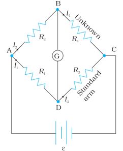
Fig. 3.25
The bridge has four resistors R1, R2, R3 and R4. Across one pair of diagonally opposite points (A and C in the figure) a source is connected. This (i.e., AC) is called the battery arm. Between the other two vertices, B and D, a galvanometer G (which is a device to detect currents) is connected. This line, shown as BD in the figure, is called the galvanometer arm.
For simplicity, we assume that the cell has no internal resistance. In general there will be currents flowing across all the resistors as well as a current Ig through G. Of special interest, is the case of a balanced bridge where the resistors are such that Ig = 0. We can easily get the balance condition, such that there is no current through G. In this case, the Kirchhoff’s junction rule applied to junctions D and B (see the figure) immediately gives us the relations I1 = I3 and I2 = I4. Next, we apply Kirchhoff’s loop rule to closed loops ADBA and CBDC. The first loop given
–I1 R1 + 0 + I2 R2 = 0 (Ig = 0) (3.81)
and the second loop gives, upon using I3 = I1, I4 = I2
I2 R4 + 0 – I1 R3 = 0 (3.82)
From Eq. (3.81), we obtain,
\(% MathType!MTEF!2!1!+- % feaagKart1ev2aaatCvAUfeBSjuyZL2yd9gzLbvyNv2CaerbuLwBLn % hiov2DGi1BTfMBaeXatLxBI9gBaerbd9wDYLwzYbItLDharqqtubsr % 4rNCHbGeaGqiVu0Je9sqqrpepC0xbbL8F4rqqrFfpeea0xe9Lq-Jc9 % vqaqpepm0xbba9pwe9Q8fs0-yqaqpepae9pg0FirpepeKkFr0xfr-x % fr-xb9adbaqaaeGaciGaaiaabeqaamaabaabaaGcbaWaaSaaaeaaca % WGjbWaaSbaaSqaaiaaigdaaeqaaaGcbaGaamysamaaBaaaleaacaaI % YaaabeaaaaGccqGH9aqpdaWcaaqaaiaadkfadaWgaaWcbaGaaGOmaa % qabaaakeaacaWGsbWaaSbaaSqaaiaaigdaaeqaaaaaaaa!3E22! \frac{{{I_1}}}{{{I_2}}} = \frac{{{R_2}}}{{{R_1}}}\)
whereas from Eq. (3.82), we obtain,
\(% MathType!MTEF!2!1!+- % feaagKart1ev2aaatCvAUfeBSjuyZL2yd9gzLbvyNv2CaerbuLwBLn % hiov2DGi1BTfMBaeXatLxBI9gBaerbd9wDYLwzYbItLDharqqtubsr % 4rNCHbGeaGqiVu0Je9sqqrpepC0xbbL8F4rqqrFfpeea0xe9Lq-Jc9 % vqaqpepm0xbba9pwe9Q8fs0-yqaqpepae9pg0FirpepeKkFr0xfr-x % fr-xb9adbaqaaeGaciGaaiaabeqaamaabaabaaGcbaWaaSaaaeaaca % WGjbWaaSbaaSqaaiaaigdaaeqaaaGcbaGaamysamaaBaaaleaacaaI % YaaabeaaaaGccqGH9aqpdaWcaaqaaiaadkfadaWgaaWcbaGaaGinaa % qabaaakeaacaWGsbWaaSbaaSqaaiaaiodaaeqaaaaaaaa!3E26! \frac{{{I_1}}}{{{I_2}}} = \frac{{{R_4}}}{{{R_3}}}\)
Hence, we obtain the condition
\(% MathType!MTEF!2!1!+- % feaagKart1ev2aaatCvAUfeBSjuyZL2yd9gzLbvyNv2CaerbuLwBLn % hiov2DGi1BTfMBaeXatLxBI9gBaerbd9wDYLwzYbItLDharqqtubsr % 4rNCHbGeaGqiVu0Je9sqqrpepC0xbbL8F4rqqrFfpeea0xe9Lq-Jc9 % vqaqpepm0xbba9pwe9Q8fs0-yqaqpepae9pg0FirpepeKkFr0xfr-x % fr-xb9adbaqaaeGaciGaaiaabeqaamaabaabaaGcbaWaaSaaaeaaca % WGsbWaaSbaaSqaaiaaikdaaeqaaaGcbaGaamOuamaaBaaaleaacaaI % XaaabeaaaaGccqGH9aqpdaWcaaqaaiaadkfadaWgaaWcbaGaaGinaa % qabaaakeaacaWGsbWaaSbaaSqaaiaaiodaaeqaaaaaaaa!3E38! \frac{{{R_2}}}{{{R_1}}} = \frac{{{R_4}}}{{{R_3}}}\) (3.83.(a))
This last equation relating the four resistors is called the balance condition for the galvanometer to give zero or null deflection.
The Wheatstone bridge and its balance condition provide a practical method for determination of an unknown resistance. Let us suppose we have an unknown resistance, which we insert in the fourth arm; R4 is thus not known. Keeping known resistances R1 and R2 in the first and second arm of the bridge, we go on varying R3 till the galvanometer shows a null deflection. The bridge then is balanced, and from the balance condition the value of the unknown resistance R4 is given by,
\(% MathType!MTEF!2!1!+- % feaagKart1ev2aaatCvAUfeBSjuyZL2yd9gzLbvyNv2CaerbuLwBLn % hiov2DGi1BTfMBaeXatLxBI9gBaerbd9wDYLwzYbItLDharqqtubsr % 4rNCHbGeaGqiVu0Je9sqqrpepC0xbbL8F4rqqrFfpeea0xe9Lq-Jc9 % vqaqpepm0xbba9pwe9Q8fs0-yqaqpepae9pg0FirpepeKkFr0xfr-x % fr-xb9adbaqaaeGaciGaaiaabeqaamaabaabaaGcbaWaaSaaaeaaca % WGsbWaaSbaaSqaaiaaikdaaeqaaaGcbaGaamOuamaaBaaaleaacaaI % XaaabeaaaaGccqGH9aqpdaWcaaqaaiaadkfadaWgaaWcbaGaaGinaa % qabaaakeaacaWGsbWaaSbaaSqaaiaaigdaaeqaaaaaaaa!3E36! \frac{{{R_2}}}{{{R_1}}} = \frac{{{R_4}}}{{{R_1}}}\) [3.83(b)]
A practical device using this principle is called the meter bridge. It will be discussed in the next section.
EXAMPLE 8
The four arms of a Wheatstone bridge (Fig. 3.26) have the following resistances:
AB = 100\(% MathType!MTEF!2!1!+- % feaagKart1ev2aaatCvAUfeBSjuyZL2yd9gzLbvyNv2CaerbuLwBLn % hiov2DGi1BTfMBaeXatLxBI9gBaerbd9wDYLwzYbItLDharqqtubsr % 4rNCHbGeaGqiVu0Je9sqqrpepC0xbbL8F4rqqrFfpeea0xe9Lq-Jc9 % vqaqpepm0xbba9pwe9Q8fs0-yqaqpepae9pg0FirpepeKkFr0xfr-x % fr-xb9adbaqaaeGaciGaaiaabeqaamaabaabaaGcbaGaeyyQdCfaaa!3785! \Omega \), BC = 10\(% MathType!MTEF!2!1!+- % feaagKart1ev2aaatCvAUfeBSjuyZL2yd9gzLbvyNv2CaerbuLwBLn % hiov2DGi1BTfMBaeXatLxBI9gBaerbd9wDYLwzYbItLDharqqtubsr % 4rNCHbGeaGqiVu0Je9sqqrpepC0xbbL8F4rqqrFfpeea0xe9Lq-Jc9 % vqaqpepm0xbba9pwe9Q8fs0-yqaqpepae9pg0FirpepeKkFr0xfr-x % fr-xb9adbaqaaeGaciGaaiaabeqaamaabaabaaGcbaGaeyyQdCfaaa!3785! \Omega \), CD = 5 \(% MathType!MTEF!2!1!+- % feaagKart1ev2aaatCvAUfeBSjuyZL2yd9gzLbvyNv2CaerbuLwBLn % hiov2DGi1BTfMBaeXatLxBI9gBaerbd9wDYLwzYbItLDharqqtubsr % 4rNCHbGeaGqiVu0Je9sqqrpepC0xbbL8F4rqqrFfpeea0xe9Lq-Jc9 % vqaqpepm0xbba9pwe9Q8fs0-yqaqpepae9pg0FirpepeKkFr0xfr-x % fr-xb9adbaqaaeGaciGaaiaabeqaamaabaabaaGcbaGaeyyQdCfaaa!3785! \Omega \) , and DA = 60\(% MathType!MTEF!2!1!+- % feaagKart1ev2aaatCvAUfeBSjuyZL2yd9gzLbvyNv2CaerbuLwBLn % hiov2DGi1BTfMBaeXatLxBI9gBaerbd9wDYLwzYbItLDharqqtubsr % 4rNCHbGeaGqiVu0Je9sqqrpepC0xbbL8F4rqqrFfpeea0xe9Lq-Jc9 % vqaqpepm0xbba9pwe9Q8fs0-yqaqpepae9pg0FirpepeKkFr0xfr-x % fr-xb9adbaqaaeGaciGaaiaabeqaamaabaabaaGcbaGaeyyQdCfaaa!3785! \Omega \).
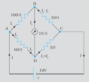
Fig. 3.26
A galvanometer of 15\(% MathType!MTEF!2!1!+- % feaagKart1ev2aaatCvAUfeBSjuyZL2yd9gzLbvyNv2CaerbuLwBLn % hiov2DGi1BTfMBaeXatLxBI9gBaerbd9wDYLwzYbItLDharqqtubsr % 4rNCHbGeaGqiVu0Je9sqqrpepC0xbbL8F4rqqrFfpeea0xe9Lq-Jc9 % vqaqpepm0xbba9pwe9Q8fs0-yqaqpepae9pg0FirpepeKkFr0xfr-x % fr-xb9adbaqaaeGaciGaaiaabeqaamaabaabaaGcbaGaeyyQdCfaaa!3785! \Omega \) resistance is connected across BD. Calculate the current through the galvanometer when a potential difference of 10 V is maintained across AC.
SOLUTION
Considering the mesh BADB, we have
100I1 + 15Ig – 60I2 = 0 or 20I1 + 3Ig – 12I2= 0
Considering the mesh BCDB, we have 10 (I1 – Ig) – 15Ig – 5 (I2 + Ig ) = 0
10I1 – 30Ig –5I2 = 0
2I1 – 6Ig – I2 = 0
Considering the mesh ADCEA, 60I2 + 5 (I2 + Ig ) = 10
65I2 + 5Ig = 10
13I2 + Ig = 2
Multiplying Eq. (3.84b) by 10
20I1 – 60Ig – 10I2 = 0 [3.84(d)]
From Eqs. (3.84d) and (3.84a) we have 63Ig – 2I2 = 0
I2 = 31.5Ig [3.84(e)]
Substituting the value of I2 into Eq. [3.84(c)],
we get 13 (31.5Ig) + Ig = 2
410.5 Ig = 2
Ig = 4.87 mA.
METER BRIDGE
The meter bridge is shown in Fig. 3.27.
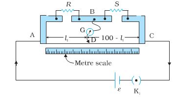
FIGURE 3.27 A meter bridge. Wire AC is 1 m long. R is a resistance to be measured and S is a standard resistance.
It consists of a wire of length 1 m and of uniform cross sectional area stretched taut and clamped between two thick metallic strips bent at right angles, as shown. The metallic strip has two gaps across which resistors can be connected. The end points where the wire is clamped are connected to a cell through a key. One end of a galvanometer is connected to the metallic strip midway between the two gaps. The other end of the galvanometer is connected to a ‘jockey’. The jockey is essentially a metallic rod whose one end has a knife-edge which can slide over the wire to make electrical connection.
R is an unknown resistance whose value we want to determine. It is connected across one of the gaps. Across the other gap, we connect a standard known resistance S. The jockey is connected to some point D on the wire, a distance l cm from the end A. The jockey can be moved along the wire. The portion AD of the wire has a resistance Rcml, where Rcm is the resistance of the wire per unit centimetre. The portion DC of the wire similarly has a resistance Rcm (100-l ).
The four arms AB, BC, DA and CD [with resistances R, S, Rcm l and Rcm(100-l )] obviously form a Wheatstone bridge with AC as the battery arm and BD the galvanometer arm. If the jockey is moved along the wire, then there will be one position where the galvanometer will show no current. Let the distance of the jockey from the end A at the balance point be l= l1. The four resistances of the bridge at the balance point then are R, S, Rcm l1 and Rcm(100–l1). The balance condition, Eq. [3.83(a)]
\(% MathType!MTEF!2!1!+- % feaagKart1ev2aaatCvAUfeBSjuyZL2yd9gzLbvyNv2CaerbuLwBLn % hiov2DGi1BTfMBaeXatLxBI9gBaerbd9wDYLwzYbItLDharqqtubsr % 4rNCHbGeaGqiVu0Je9sqqrpepC0xbbL8F4rqqrFfpeea0xe9Lq-Jc9 % vqaqpepm0xbba9pwe9Q8fs0-yqaqpepae9pg0FirpepeKkFr0xfr-x % fr-xb9adbaqaaeGaciGaaiaabeqaamaabaabaaGcbaWaaSaaaeaaca % WGsbaabaGaam4uaaaacqGH9aqpdaWcaaqaaiaadkfadaWgaaWcbaGa % am4yaiaad2gaaeqaaOGaamiBamaaBaaaleaacaaIYaaabeaaaOqaai % aadkfadaWgaaWcbaGaam4yaiaad2gaaeqaaOGaaiikaiaaigdacaaI % WaGaaGimaiabgkHiTiaadYgadaWgaaWcbaGaaGymaaqabaGccaGGPa % aaaiabg2da9maalaaabaGaamiBamaaBaaaleaacaaIXaaabeaaaOqa % aiaaigdacaaIWaGaaGimaiabgkHiTiaadYgadaWgaaWcbaGaaGymaa % qabaaaaaaa!4EBF! \frac{R}{S} = \frac{{{R_{cm}}{l_2}}}{{{R_{cm}}(100 - {l_1})}} = \frac{{{l_1}}}{{100 - {l_1}}}\) (3.85)
Thus, once we have found out l1, the unknown resistance R is known in terms of the standard known resistance S by
\(% MathType!MTEF!2!1!+- % feaagKart1ev2aaatCvAUfeBSjuyZL2yd9gzLbvyNv2CaerbuLwBLn % hiov2DGi1BTfMBaeXatLxBI9gBaerbd9wDYLwzYbItLDharqqtubsr % 4rNCHbGeaGqiVu0Je9sqqrpepC0xbbL8F4rqqrFfpeea0xe9Lq-Jc9 % vqaqpepm0xbba9pwe9Q8fs0-yqaqpepae9pg0FirpepeKkFr0xfr-x % fr-xb9adbaqaaeGaciGaaiaabeqaamaabaabaaGcbaGaamOuaiabg2 % da9iaadofadaWcaaqaaiaadYgadaWgaaWcbaGaaGymaaqabaaakeaa % caaIXaGaaGimaiaaicdacqGHsislcaWGSbWaaSbaaSqaaiaaigdaae % qaaaaaaaa!3F91! R = S\frac{{{l_1}}}{{100 - {l_1}}}\) (3.86)
By choosing various values of S, we would get various values of l1, and calculate R each time. An error in measurement of l1 would naturally result in an error in R. It can be shown that the percentage error in R can be minimised by adjusting the balance point near the middle of the
bridge, i.e., when l1 is close to 50 cm. ( This requires a suitable choice of S.)
EXAMPLE 9
In a meter bridge (Fig. 3.27), the null point is found at a distance of 33.7 cm from A. If now a resistance of 12\(% MathType!MTEF!2!1!+- % feaagKart1ev2aaatCvAUfeBSjuyZL2yd9gzLbvyNv2CaerbuLwBLn % hiov2DGi1BTfMBaeXatLxBI9gBaerbd9wDYLwzYbItLDharqqtubsr % 4rNCHbGeaGqiVu0Je9sqqrpepC0xbbL8F4rqqrFfpeea0xe9Lq-Jc9 % vqaqpepm0xbba9pwe9Q8fs0-yqaqpepae9pg0FirpepeKkFr0xfr-x % fr-xb9adbaqaaeGaciGaaiaabeqaamaabaabaaGcbaGaeyyQdCfaaa!3785! \Omega \) is connected in parallel with S, the null point occurs at 51.9 cm. Determine the values of R and S.
SOLUTION
From the first balance point, we get \(% MathType!MTEF!2!1!+- % feaagKart1ev2aaatCvAUfeBSjuyZL2yd9gzLbvyNv2CaerbuLwBLn % hiov2DGi1BTfMBaeXatLxBI9gBaerbd9wDYLwzYbItLDharqqtubsr % 4rNCHbGeaGqiVu0Je9sqqrpepC0xbbL8F4rqqrFfpeea0xe9Lq-Jc9 % vqaqpepm0xbba9pwe9Q8fs0-yqaqpepae9pg0FirpepeKkFr0xfr-x % fr-xb9adbaqaaeGaciGaaiaabeqaamaabaabaaGcbaWaaSaaaeaaca % WGsbaabaGaam4uaaaacqGH9aqpdaWcaaqaaiaaiodacaaIZaGaaiOl % aiaaiEdaaeaacaaI2aGaaGOnaiaac6cacaaIZaaaaaaa!3EA7! \frac{R}{S} = \frac{{33.7}}{{66.3}}\)
After S is connected in parallel with a resistance of 12\(% MathType!MTEF!2!1!+- % feaagKart1ev2aaatCvAUfeBSjuyZL2yd9gzLbvyNv2CaerbuLwBLn % hiov2DGi1BTfMBaeXatLxBI9gBaerbd9wDYLwzYbItLDharqqtubsr % 4rNCHbGeaGqiVu0Je9sqqrpepC0xbbL8F4rqqrFfpeea0xe9Lq-Jc9 % vqaqpepm0xbba9pwe9Q8fs0-yqaqpepae9pg0FirpepeKkFr0xfr-x % fr-xb9adbaqaaeGaciGaaiaabeqaamaabaabaaGcbaGaeyyQdCfaaa!3785! \Omega \), the resistance across the gap changes from S to Seq, where
\(% MathType!MTEF!2!1!+- % feaagKart1ev2aaatCvAUfeBSjuyZL2yd9gzLbvyNv2CaerbuLwBLn % hiov2DGi1BTfMBaeXatLxBI9gBaerbd9wDYLwzYbItLDharqqtubsr % 4rNCHbGeaGqiVu0Je9sqqrpepC0xbbL8F4rqqrFfpeea0xe9Lq-Jc9 % vqaqpepm0xbba9pwe9Q8fs0-yqaqpepae9pg0FirpepeKkFr0xfr-x % fr-xb9adbaqaaeGaciGaaiaabeqaamaabaabaaGcbaGaam4uamaaBa % aaleaacaWGLbGaamyCaaqabaGccqGH9aqpdaWcaaqaaiaaigdacaaI % YaGaam4uaaqaaiaadofacqGHRaWkcaaIXaGaaGOmaaaaaaa!3F7A! {S_{eq}} = \frac{{12S}}{{S + 12}}\) (3.87)
and hence the new balance condition now gives
\(% MathType!MTEF!2!1!+- % feaagKart1ev2aaatCvAUfeBSjuyZL2yd9gzLbvyNv2CaerbuLwBLn % hiov2DGi1BTfMBaeXatLxBI9gBaerbd9wDYLwzYbItLDharqqtubsr % 4rNCHbGeaGqiVu0Je9sqqrpepC0xbbL8F4rqqrFfpeea0xe9Lq-Jc9 % vqaqpepm0xbba9pwe9Q8fs0-yqaqpepae9pg0FirpepeKkFr0xfr-x % fr-xb9adbaqaaeGaciGaaiaabeqaamaabaabaaGcbaWaaSaaaeaaca % aI1aGaaGymaiaac6cacaaI5aaabaGaaGinaiaaiIdacaGGUaGaaGym % aaaacqGH9aqpdaWcaaqaaiaadkfaaeaacaWGtbWaaSbaaSqaaiaadw % gacaWGXbaabeaaaaGccqGH9aqpdaWcaaqaaiaadkfadaqadaqaaiaa % dofacqGHRaWkcaaIXaGaaGOmaaGaayjkaiaawMcaaiaaigdacaaIYa % Gaam4uaaqaaiaaigdacaaIYaGaam4uaaaaaaa!4C02! \frac{{51.9}}{{48.1}} = \frac{R}{{{S_{eq}}}} = \frac{{R\left( {S + 12} \right)12S}}{{12S}}\) (3.88)
Substituting the value of R/S from Eq. (3.87), we get
\(% MathType!MTEF!2!1!+- % feaagKart1ev2aaatCvAUfeBSjuyZL2yd9gzLbvyNv2CaerbuLwBLn % hiov2DGi1BTfMBaeXatLxBI9gBaerbd9wDYLwzYbItLDharqqtubsr % 4rNCHbGeaGqiVu0Je9sqqrpepC0xbbL8F4rqqrFfpeea0xe9Lq-Jc9 % vqaqpepm0xbba9pwe9Q8fs0-yqaqpepae9pg0FirpepeKkFr0xfr-x % fr-xb9adbaqaaeGaciGaaiaabeqaamaabaabaaGcbaWaaSaaaeaaca % aI1aGaaGymaiaac6cacaaI5aaabaGaaGinaiaaiIdacaGGUaGaaGym % aaaacqGH9aqpdaWcaaqaaiaadofacqGHRaWkcaaIXaGaaGOmaaqaai % aaigdacaaIYaaaaiaac6cadaWcaaqaaiaaiodacaaIZaGaaiOlaiaa % iEdaaeaacaaI2aGaaGOnaiaac6cacaaIZaaaaaaa!483E! \frac{{51.9}}{{48.1}} = \frac{{S + 12}}{{12}}.\frac{{33.7}}{{66.3}}\)
which gives S = 13.5\(% MathType!MTEF!2!1!+- % feaagKart1ev2aaatCvAUfeBSjuyZL2yd9gzLbvyNv2CaerbuLwBLn % hiov2DGi1BTfMBaeXatLxBI9gBaerbd9wDYLwzYbItLDharqqtubsr % 4rNCHbGeaGqiVu0Je9sqqrpepC0xbbL8F4rqqrFfpeea0xe9Lq-Jc9 % vqaqpepm0xbba9pwe9Q8fs0-yqaqpepae9pg0FirpepeKkFr0xfr-x % fr-xb9adbaqaaeGaciGaaiaabeqaamaabaabaaGcbaGaeyyQdCfaaa!3785! \Omega \). Using the value of R/S above, we get R = 6.86 \(% MathType!MTEF!2!1!+- % feaagKart1ev2aaatCvAUfeBSjuyZL2yd9gzLbvyNv2CaerbuLwBLn % hiov2DGi1BTfMBaeXatLxBI9gBaerbd9wDYLwzYbItLDharqqtubsr % 4rNCHbGeaGqiVu0Je9sqqrpepC0xbbL8F4rqqrFfpeea0xe9Lq-Jc9 % vqaqpepm0xbba9pwe9Q8fs0-yqaqpepae9pg0FirpepeKkFr0xfr-x % fr-xb9adbaqaaeGaciGaaiaabeqaamaabaabaaGcbaGaeyyQdCfaaa!3785! \Omega \).
POTENTIOMETER
This is a versatile instrument. It is basically a long piece of uniform wire, sometimes a few meters in length across which a standard cell (B) is connected. In actual design, the wire is sometimes cut in several pieces placed side by side and connected at the ends by thick metal strip. (Fig. 3.28).
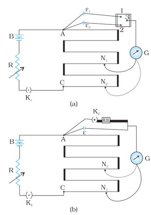
FIGURE 3.28 A potentiometer. G is a galvanometer and R a variable resistance (rheostat). 1, 2, 3 are terminals of a two way key circuit for comparing emfs of two cells; (b) circuit for determining internal resistance of a cell.
In the figure, the wires run from A to C. The small vertical portions are the thick metal strips connecting the various sections of the wire.
A current I flows through the wire which can be varied by a variable resistance (rheostat, R) in the circuit. Since the wire is uniform, the potential difference between A and any point at a distance l from A is
\(% MathType!MTEF!2!1!+- % feaagKart1ev2aaatCvAUfeBSjuyZL2yd9gzLbvyNv2CaerbuLwBLn % hiov2DGi1BTfMBaeXatLxBI9gBaerbd9wDYLwzYbItLDharqqtubsr % 4rNCHbGeaGqiVu0Je9sqqrpepC0xbbL8F4rqqrFfpeea0xe9Lq-Jc9 % vqaqpepm0xbba9pwe9Q8fs0-yqaqpepae9pg0FirpepeKkFr0xfr-x % fr-xb9adbaqaaeGaciGaaiaabeqaamaabaabaaGcbaGaeqyTdu2aae % WaaeaacaWGSbaacaGLOaGaayzkaaGaeyypa0Jaeqy1dyMaamiBaaaa % !3DD6! \varepsilon \left( l \right) = \phi l\) (3.89)
where \(% MathType!MTEF!2!1!+- % feaagKart1ev2aaatCvAUfeBSjuyZL2yd9gzLbvyNv2CaerbuLwBLn % hiov2DGi1BTfMBaeXatLxBI9gBaerbd9wDYLwzYbItLDharqqtubsr % 4rNCHbGeaGqiVu0Je9sqqrpepC0xbbL8F4rqqrFfpeea0xe9Lq-Jc9 % vqaqpepm0xbba9pwe9Q8fs0-yqaqpepae9pg0FirpepeKkFr0xfr-x % fr-xb9adbaqaaeGaciGaaiaabeqaamaabaabaaGcbaGaeqy1dygaaa!37BE! \phi \) is the potential drop per unit length.
Figure 3.28 (a) shows an application of the potentiometer to compare the emf of two cells of emf \(% MathType!MTEF!2!1!+- % feaagKart1ev2aaatCvAUfeBSjuyZL2yd9gzLbvyNv2CaerbuLwBLn % hiov2DGi1BTfMBaeXatLxBI9gBaerbd9wDYLwzYbItLDharqqtubsr % 4rNCHbGeaGqiVu0Je9sqqrpepC0xbbL8F4rqqrFfpeea0xe9Lq-Jc9 % vqaqpepm0xbba9pwe9Q8fs0-yqaqpepae9pg0FirpepeKkFr0xfr-x % fr-xb9adbaqaaeGaciGaaiaabeqaamaabaabaaGcbaGaeqyTdugaaa!379D! \varepsilon \)1 and \(% MathType!MTEF!2!1!+- % feaagKart1ev2aaatCvAUfeBSjuyZL2yd9gzLbvyNv2CaerbuLwBLn % hiov2DGi1BTfMBaeXatLxBI9gBaerbd9wDYLwzYbItLDharqqtubsr % 4rNCHbGeaGqiVu0Je9sqqrpepC0xbbL8F4rqqrFfpeea0xe9Lq-Jc9 % vqaqpepm0xbba9pwe9Q8fs0-yqaqpepae9pg0FirpepeKkFr0xfr-x % fr-xb9adbaqaaeGaciGaaiaabeqaamaabaabaaGcbaGaeqyTdugaaa!379D! \varepsilon \)2 . The points marked 1, 2, 3 form a two way key. Consider first a position of the key where 1 and 3 are connected so that the galvanometer is connected to \(% MathType!MTEF!2!1!+- % feaagKart1ev2aaatCvAUfeBSjuyZL2yd9gzLbvyNv2CaerbuLwBLn % hiov2DGi1BTfMBaeXatLxBI9gBaerbd9wDYLwzYbItLDharqqtubsr % 4rNCHbGeaGqiVu0Je9sqqrpepC0xbbL8F4rqqrFfpeea0xe9Lq-Jc9 % vqaqpepm0xbba9pwe9Q8fs0-yqaqpepae9pg0FirpepeKkFr0xfr-x % fr-xb9adbaqaaeGaciGaaiaabeqaamaabaabaaGcbaGaeqyTdugaaa!379D! \varepsilon \)1. The jockey is moved along the wire till at a point N1, at a distance l1 from A, there is no deflection in the galvanometer. We can apply Kirchhoff’s loop rule to the closed loop AN1G31A and get
\(% MathType!MTEF!2!1!+- % feaagKart1ev2aaatCvAUfeBSjuyZL2yd9gzLbvyNv2CaerbuLwBLn % hiov2DGi1BTfMBaeXatLxBI9gBaerbd9wDYLwzYbItLDharqqtubsr % 4rNCHbGeaGqiVu0Je9sqqrpepC0xbbL8F4rqqrFfpeea0xe9Lq-Jc9 % vqaqpepm0xbba9pwe9Q8fs0-yqaqpepae9pg0FirpepeKkFr0xfr-x % fr-xb9adbaqaaeGaciGaaiaabeqaamaabaabaaGcbaGaeqy1dyMaam % iBamaaBaaaleaacaaIXaaabeaakiabgUcaRiaaicdacqGHsislcqaH % 1oqzdaWgaaWcbaGaaGymaaqabaGccqGH9aqpcaaIWaaaaa!4081! \phi {l_1} + 0 - {\varepsilon _1} = 0\)(3.90)
Similarly, if another emf \(% MathType!MTEF!2!1!+- % feaagKart1ev2aaatCvAUfeBSjuyZL2yd9gzLbvyNv2CaerbuLwBLn % hiov2DGi1BTfMBaeXatLxBI9gBaerbd9wDYLwzYbItLDharqqtubsr % 4rNCHbGeaGqiVu0Je9sqqrpepC0xbbL8F4rqqrFfpeea0xe9Lq-Jc9 % vqaqpepm0xbba9pwe9Q8fs0-yqaqpepae9pg0FirpepeKkFr0xfr-x % fr-xb9adbaqaaeGaciGaaiaabeqaamaabaabaaGcbaGaeqyTdugaaa!379D! \varepsilon \)2 is balanced against l2 (AN2)
\(% MathType!MTEF!2!1!+- % feaagKart1ev2aaatCvAUfeBSjuyZL2yd9gzLbvyNv2CaerbuLwBLn % hiov2DGi1BTfMBaeXatLxBI9gBaerbd9wDYLwzYbItLDharqqtubsr % 4rNCHbGeaGqiVu0Je9sqqrpepC0xbbL8F4rqqrFfpeea0xe9Lq-Jc9 % vqaqpepm0xbba9pwe9Q8fs0-yqaqpepae9pg0FirpepeKkFr0xfr-x % fr-xb9adbaqaaeGaciGaaiaabeqaamaabaabaaGcbaGaeqy1dyMaam % iBamaaBaaaleaacaaIXaaabeaakiabgUcaRiaaicdacqGHsislcqaH % 1oqzdaWgaaWcbaGaaGymaaqabaGccqGH9aqpcaaIWaaaaa!4081! \phi {l_2} + 0 - {\varepsilon _2} = 0\) (3.91)
From the last two equations
\(% MathType!MTEF!2!1!+- % feaagKart1ev2aaatCvAUfeBSjuyZL2yd9gzLbvyNv2CaerbuLwBLn % hiov2DGi1BTfMBaeXatLxBI9gBaerbd9wDYLwzYbItLDharqqtubsr % 4rNCHbGeaGqiVu0Je9sqqrpepC0xbbL8F4rqqrFfpeea0xe9Lq-Jc9 % vqaqpepm0xbba9pwe9Q8fs0-yqaqpepae9pg0FirpepeKkFr0xfr-x % fr-xb9adbaqaaeGaciGaaiaabeqaamaabaabaaGcbaWaaSaaaeaacq % aH1oqzdaWgaaWcbaGaaGymaaqabaaakeaacqaH1oqzdaWgaaWcbaGa % aGOmaaqabaaaaOGaeyypa0ZaaSaaaeaacaWGSbWaaSbaaSqaaiaaig % daaeqaaaGcbaGaamiBamaaBaaaleaacaaIYaaabeaaaaaaaa!4008! \frac{{{\varepsilon _1}}}{{{\varepsilon _2}}} = \frac{{{l_1}}}{{{l_2}}}\) (3.92)
This simple mechanism thus allows one to compare the emf’s of any two sources (\(% MathType!MTEF!2!1!+- % feaagKart1ev2aaatCvAUfeBSjuyZL2yd9gzLbvyNv2CaerbuLwBLn % hiov2DGi1BTfMBaeXatLxBI9gBaerbd9wDYLwzYbItLDharqqtubsr % 4rNCHbGeaGqiVu0Je9sqqrpepC0xbbL8F4rqqrFfpeea0xe9Lq-Jc9 % vqaqpepm0xbba9pwe9Q8fs0-yqaqpepae9pg0FirpepeKkFr0xfr-x % fr-xb9adbaqaaeGaciGaaiaabeqaamaabaabaaGcbaGaeqyTdugaaa!379D! \varepsilon \)1,\(% MathType!MTEF!2!1!+- % feaagKart1ev2aaatCvAUfeBSjuyZL2yd9gzLbvyNv2CaerbuLwBLn % hiov2DGi1BTfMBaeXatLxBI9gBaerbd9wDYLwzYbItLDharqqtubsr % 4rNCHbGeaGqiVu0Je9sqqrpepC0xbbL8F4rqqrFfpeea0xe9Lq-Jc9 % vqaqpepm0xbba9pwe9Q8fs0-yqaqpepae9pg0FirpepeKkFr0xfr-x % fr-xb9adbaqaaeGaciGaaiaabeqaamaabaabaaGcbaGaeqyTdugaaa!379D! \varepsilon \)2). In practice one of the cells is chosen as a standard cell whose emf is known to a high degree of accuracy. The emf of the other cell is then easily calculated from Eq. (3.92).
We can also use a potentiometer to measure internal resistance of a cell [Fig. 3.28 (b)]. For this the cell (emf \(% MathType!MTEF!2!1!+- % feaagKart1ev2aaatCvAUfeBSjuyZL2yd9gzLbvyNv2CaerbuLwBLn % hiov2DGi1BTfMBaeXatLxBI9gBaerbd9wDYLwzYbItLDharqqtubsr % 4rNCHbGeaGqiVu0Je9sqqrpepC0xbbL8F4rqqrFfpeea0xe9Lq-Jc9 % vqaqpepm0xbba9pwe9Q8fs0-yqaqpepae9pg0FirpepeKkFr0xfr-x % fr-xb9adbaqaaeGaciGaaiaabeqaamaabaabaaGcbaGaeqyTdugaaa!379D! \varepsilon \) ) whose internal resistance (r) is to be determined is connected across a resistance box through a key K2, as shown in the figure. With key K2 open, balance is obtained at length l1 (AN1). Then,
\(% MathType!MTEF!2!1!+- % feaagKart1ev2aaatCvAUfeBSjuyZL2yd9gzLbvyNv2CaerbuLwBLn % hiov2DGi1BTfMBaeXatLxBI9gBaerbd9wDYLwzYbItLDharqqtubsr % 4rNCHbGeaGqiVu0Je9sqqrpepC0xbbL8F4rqqrFfpeea0xe9Lq-Jc9 % vqaqpepm0xbba9pwe9Q8fs0-yqaqpepae9pg0FirpepeKkFr0xfr-x % fr-xb9adbaqaaeGaciGaaiaabeqaamaabaabaaGcbaGaeqyTduMaey % ypa0Jaeqy1dyMaamiBamaaBaaaleaacaaIXaaabeaaaaa!3C43! \varepsilon = \phi {l_1}\) (3.93(a))
When key K2 is closed, the cell sends a current (I ) through the resistance box (R). If V is the terminal potential difference of the cell and balance is obtained at length l2 (AN2),
\(% MathType!MTEF!2!1!+- % feaagKart1ev2aaatCvAUfeBSjuyZL2yd9gzLbvyNv2CaerbuLwBLn % hiov2DGi1BTfMBaeXatLxBI9gBaerbd9wDYLwzYbItLDharqqtubsr % 4rNCHbGeaGqiVu0Je9sqqrpepC0xbbL8F4rqqrFfpeea0xe9Lq-Jc9 % vqaqpepm0xbba9pwe9Q8fs0-yqaqpepae9pg0FirpepeKkFr0xfr-x % fr-xb9adbaqaaeGaciGaaiaabeqaamaabaabaaGcbaGaamOvaiabg2 % da9iabew9aMjaadYgadaWgaaWcbaGaaGOmaaqabaaaaa!3B78! V = \phi {l_2}\) (3.94(b))
So, we have \(% MathType!MTEF!2!1!+- % feaagKart1ev2aaatCvAUfeBSjuyZL2yd9gzLbvyNv2CaerbuLwBLn % hiov2DGi1BTfMBaeXatLxBI9gBaerbd9wDYLwzYbItLDharqqtubsr % 4rNCHbGeaGqiVu0Je9sqqrpepC0xbbL8F4rqqrFfpeea0xe9Lq-Jc9 % vqaqpepm0xbba9pwe9Q8fs0-yqaqpepae9pg0FirpepeKkFr0xfr-x % fr-xb9adbaqaaeGaciGaaiaabeqaamaabaabaaGcbaGaeqyTdugaaa!379D! \varepsilon \)/V = l1/l 2 [3.94(a)]
But, \(% MathType!MTEF!2!1!+- % feaagKart1ev2aaatCvAUfeBSjuyZL2yd9gzLbvyNv2CaerbuLwBLn % hiov2DGi1BTfMBaeXatLxBI9gBaerbd9wDYLwzYbItLDharqqtubsr % 4rNCHbGeaGqiVu0Je9sqqrpepC0xbbL8F4rqqrFfpeea0xe9Lq-Jc9 % vqaqpepm0xbba9pwe9Q8fs0-yqaqpepae9pg0FirpepeKkFr0xfr-x % fr-xb9adbaqaaeGaciGaaiaabeqaamaabaabaaGcbaGaeqyTdugaaa!379D! \varepsilon \) = I (r + R ) and V = IR. This gives
\(% MathType!MTEF!2!1!+- % feaagKart1ev2aaatCvAUfeBSjuyZL2yd9gzLbvyNv2CaerbuLwBLn % hiov2DGi1BTfMBaeXatLxBI9gBaerbd9wDYLwzYbItLDharqqtubsr % 4rNCHbGeaGqiVu0Je9sqqrpepC0xbbL8F4rqqrFfpeea0xe9Lq-Jc9 % vqaqpepm0xbba9pwe9Q8fs0-yqaqpepae9pg0FirpepeKkFr0xfr-x % fr-xb9adbaqaaeGaciGaaiaabeqaamaabaabaaGcbaGaeqyTdugaaa!379D! \varepsilon \)/V = (r+R )/R [3.94(b)]
From Eq. [3.94(a)] and [3.94(b)]
we have (R+r )/R = l1/l 2
\(% MathType!MTEF!2!1!+- % feaagKart1ev2aaatCvAUfeBSjuyZL2yd9gzLbvyNv2CaerbuLwBLn % hiov2DGi1BTfMBaeXatLxBI9gBaerbd9wDYLwzYbItLDharqqtubsr % 4rNCHbGeaGqiVu0Je9sqqrpepC0xbbL8F4rqqrFfpeea0xe9Lq-Jc9 % vqaqpepm0xbba9pwe9Q8fs0-yqaqpepae9pg0FirpepeKkFr0xfr-x % fr-xb9adbaqaaeGaciGaaiaabeqaamaabaabaaGcbaGaamOCaiabg2 % da9iaadkfadaqadaqaamaalaaabaGaamiBamaaBaaaleaacaaIXaaa % beaaaOqaaiaadYgadaWgaaWcbaGaaGOmaaqabaaaaOGaeyOeI0IaaG % ymaaGaayjkaiaawMcaaaaa!3FD0! r = R\left( {\frac{{{l_1}}}{{{l_2}}} - 1} \right)\) (3.95)
Using Eq. (3.95) we can find the internal resistance of a given cell. The potentiometer has the advantage that it draws no current from the voltage source being measured. As such it is unaffected by the internal resistance of the source.
EXAMPLE 10
A resistance of R \(% MathType!MTEF!2!1!+- % feaagKart1ev2aaatCvAUfeBSjuyZL2yd9gzLbvyNv2CaerbuLwBLn % hiov2DGi1BTfMBaeXatLxBI9gBaerbd9wDYLwzYbItLDharqqtubsr % 4rNCHbGeaGqiVu0Je9sqqrpepC0xbbL8F4rqqrFfpeea0xe9Lq-Jc9 % vqaqpepm0xbba9pwe9Q8fs0-yqaqpepae9pg0FirpepeKkFr0xfr-x % fr-xb9adbaqaaeGaciGaaiaabeqaamaabaabaaGcbaGaeyyQdCfaaa!3785! \Omega \) draws current from a potentiometer. The potentiometer has a total resistance R0 \(% MathType!MTEF!2!1!+- % feaagKart1ev2aaatCvAUfeBSjuyZL2yd9gzLbvyNv2CaerbuLwBLn % hiov2DGi1BTfMBaeXatLxBI9gBaerbd9wDYLwzYbItLDharqqtubsr % 4rNCHbGeaGqiVu0Je9sqqrpepC0xbbL8F4rqqrFfpeea0xe9Lq-Jc9 % vqaqpepm0xbba9pwe9Q8fs0-yqaqpepae9pg0FirpepeKkFr0xfr-x % fr-xb9adbaqaaeGaciGaaiaabeqaamaabaabaaGcbaGaeyyQdCfaaa!3785! \Omega \) (Fig. 3.29). A voltage V is supplied to the potentiometer. Derive an expression for the voltage across R when the sliding contact is in the middle of the potentiometer.
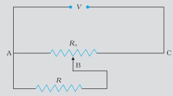
Fig. 3.29
SOLUTION
While the slide is in the middle of the potentiometer only half of its resistance (R0/2) will be between the points A and B. Hence, the total resistance between A and B, say, R1, will be given by the following expression:
\(% MathType!MTEF!2!1!+- % feaagKart1ev2aaatCvAUfeBSjuyZL2yd9gzLbvyNv2CaerbuLwBLn % hiov2DGi1BTfMBaeXatLxBI9gBaerbd9wDYLwzYbItLDharqqtubsr % 4rNCHbGeaGqiVu0Je9sqqrpepC0xbbL8F4rqqrFfpeea0xe9Lq-Jc9 % vqaqpepm0xbba9pwe9Q8fs0-yqaqpepae9pg0FirpepeKkFr0xfr-x % fr-xb9adbaqaaeGaciGaaiaabeqaamaabaabaaGceaqabeaadaWcaa % qaaiaaigdaaeaacaWGsbWaaSbaaSqaaiaaigdaaeqaaaaakiabg2da % 9maalaaabaGaaGymaaqaaiaadkfaaaGaey4kaSYaaSaaaeaacaaIXa % aabaWaaeWaaeaacaWGsbWaaSbaaSqaaiaaicdaaeqaaOGaai4laiaa % ikdaaiaawIcacaGLPaaaaaaabaGaamOuamaaBaaaleaacaaIXaaabe % aakiabg2da9maalaaabaGaamOuamaaBaaaleaacaaIWaaabeaakiaa % dkfaaeaacaWGsbWaaSbaaSqaaiaaicdaaeqaaOGaey4kaSIaaGOmai % aadkfaaaaaaaa!4B5C! \begin{array}{l} \frac{1}{{{R_1}}} = \frac{1}{R} + \frac{1}{{\left( {{R_0}/2} \right)}}\\ {R_1} = \frac{{{R_0}R}}{{{R_0} + 2R}} \end{array}\)
The total resistance between A and C will be sum of resistance between A and B and B and C, i.e., R1 + R0/2
\(\therefore\) The current flowing through the potentiometer will be \(% MathType!MTEF!2!1!+- % feaagKart1ev2aaatCvAUfeBSjuyZL2yd9gzLbvyNv2CaerbuLwBLn % hiov2DGi1BTfMBaeXatLxBI9gBaerbd9wDYLwzYbItLDharqqtubsr % 4rNCHbGeaGqiVu0Je9sqqrpepC0xbbL8F4rqqrFfpeea0xe9Lq-Jc9 % vqaqpepm0xbba9pwe9Q8fs0-yqaqpepae9pg0FirpepeKkFr0xfr-x % fr-xb9adbaqaaeGaciGaaiaabeqaamaabaabaaGcbaGaamysaiabg2 % da9maalaaabaGaamOvaaqaaiaadkfadaWgaaWcbaGaaGymaaqabaGc % cqGHRaWkcaWGsbWaaSbaaSqaaiaaicdaaeqaaOGaai4laiaaikdaaa % Gaeyypa0ZaaSaaaeaacaaIYaGaamOvaaqaaiaaikdacaWGsbWaaSba % aSqaaiaaigdaaeqaaOGaamOuamaaBaaaleaacaaIWaaabeaaaaaaaa!4583! I = \frac{V}{{{R_1} + {R_0}/2}} = \frac{{2V}}{{2{R_1}{R_0}}}\)
The voltage V1 taken from the potentiometer will be the product of current I and resistance R1,
\(% MathType!MTEF!2!1!+- % feaagKart1ev2aaatCvAUfeBSjuyZL2yd9gzLbvyNv2CaerbuLwBLn % hiov2DGi1BTfMBaeXatLxBI9gBaerbd9wDYLwzYbItLDharqqtubsr % 4rNCHbGeaGqiVu0Je9sqqrpepC0xbbL8F4rqqrFfpeea0xe9Lq-Jc9 % vqaqpepm0xbba9pwe9Q8fs0-yqaqpepae9pg0FirpepeKkFr0xfr-x % fr-xb9adbaqaaeGaciGaaiaabeqaamaabaabaaGcbaGaamOvamaaBa % aaleaacaaIXaaabeaakiabg2da9iaadMeacaWGsbWaaSbaaSqaaiaa % igdaaeqaaOGaeyypa0ZaaeWaaeaadaWcaaqaaiaaikdacaWGwbaaba % GaaGOmaiaadkfadaWgaaWcbaGaaGymaaqabaGccqGHRaWkcaWGsbWa % aSbaaSqaaiaaicdaaeqaaaaaaOGaayjkaiaawMcaaiabgEna0kaadk % fadaWgaaWcbaGaaGymaaqabaaaaa!4896! {V_1} = I{R_1} = \left( {\frac{{2V}}{{2{R_1} + {R_0}}}} \right) \times {R_1}\)
Substituting for R1, we have a
\(% MathType!MTEF!2!1!+- % feaagKart1ev2aaatCvAUfeBSjuyZL2yd9gzLbvyNv2CaerbuLwBLn % hiov2DGi1BTfMBaeXatLxBI9gBaerbd9wDYLwzYbItLDharqqtubsr % 4rNCHbGeaGqiVu0Je9sqqrpepC0xbbL8F4rqqrFfpeea0xe9Lq-Jc9 % vqaqpepm0xbba9pwe9Q8fs0-yqaqpepae9pg0FirpepeKkFr0xfr-x % fr-xb9adbaqaaeGaciGaaiaabeqaamaabaabaaGceaqabeaacaWGwb % WaaSbaaSqaaiaaigdaaeqaaOGaeyypa0ZaaSaaaeaacaaIYaGaamOv % aaqaamaabmaabaWaaSaaaeaacaWGsbWaaSbaaSqaaiaaicdaaeqaaO % Gaey41aqRaamOuaaqaaiaadkfadaWgaaWcbaGaaGimaaqabaGccqGH % RaWkcaaIYaGaamOuaaaaaiaawIcacaGLPaaaaaGaey41aq7aaSaaae % aacaWGsbWaaSbaaSqaaiaaicdaaeqaaOGaey41aqRaamOuaaqaaiaa % dkfadaWgaaWcbaGaaGimaaqabaGccqGHRaWkcaaIYaGaamOuaaaaae % aacaWGwbWaaSbaaSqaaiaaigdaaeqaaOGaeyypa0ZaaSaaaeaacaaI % YaGaamOvaiaadkfaaeaacaaIYaGaamOuaiabgUcaRiaadkfadaWgaa % WcbaGaaGimaaqabaGccqGHRaWkcaaIYaGaamOuaaaaaeaacaWGVbGa % amOCaiaaykW7caaMc8UaaGPaVlaaykW7caaMc8UaamOvamaaBaaale % aacaaIXaaabeaakiabg2da9maalaaabaGaaGOmaiaadAfacaWGsbaa % baGaamOuamaaBaaaleaacaaIWaaabeaakiabgUcaRiaaisdacaWGsb % aaaaaaaa!6F4A! \begin{array}{l} {V_1} = \frac{{2V}}{{\left( {\frac{{{R_0} \times R}}{{{R_0} + 2R}}} \right)}} \times \frac{{{R_0} \times R}}{{{R_0} + 2R}}\\ {V_1} = \frac{{2VR}}{{2R + {R_0} + 2R}}\\ or\,\,\,\,\,{V_1} = \frac{{2VR}}{{{R_0} + 4R}} \end{array}\)