-
Trigonometry And Differentiation
Trigonometry And Differentiation
DIFFERENTIATION: Sir Isaac Newton and Gottfried Wilhem Leibnitz developed calculus.
Constant quantity: If the value of a quantity remains the same in a mathematical
operation, it is called a constant quantity.
Examples: Integers (4, 7, 13, ...), Fraction (1/2, 4/5), \( \pi \), e, etc.,
Variable quantity: If the quantity takes different values in a mathematical
operation, it is called a variable quantity.
Examples: (i) In the equation y = 2x + 3, x and y are variables.
(ii) In the equation F = ma where F, m and a are variables.
Variable quantities are divided into two types
(a) Independent quantity. (b) Dependent quantity.
In the equation y = 2x + 3, x is the independent quantity and y is the dependent quantity.
Function: If corresponding to any given value of x, there exists a single definite value of y, then y is called a function of x. This is represented as y = f(x). This equation means that corresponding to one value of x, there is a single definite value of the variable y.
Example : (i) Let y = 2x, when x = 1 then y = 2 ; when x = 2 then y = 4 ......
Thus corresponding to each value of x, there is a definite value of y.
Difference and Differential coefficient:
Let y be a function of x. This is denoted as y = f(x). Here x and y are variables. Let the value of x change to \( x + \Delta \,x \) and correspondingly the value of y changes to \( y + \Delta \,y \).
The change between the initial and final values of a variable quantity is called its difference.
Difference in \( x = \left( {x + \Delta \,x} \right) - x = \Delta \,x \); Difference in \( y = \left( {y + \Delta \,y} \right) - y = \Delta \,y \)
The ratio of \( \Delta \,y/\Delta \,x \) is called the quotient of the two increments.
When difference in x (i.e., \( \Delta x \)) is very very very small i.e., almost approaching to zero, then we write \( \frac{{\Delta y}} {{\Delta x}} \) is equal to \( \frac{{dy}} {{dx}} \).
In mathematical language we represent the above statement as :\( \mathop {Limit}\limits_{\Delta x \to 0} \frac{{\Delta y}} {{\Delta x}} = \frac{{dy}} {{dx}} \) or \( \mathop {Lt}\limits_{\Delta x \to 0} \frac{{\Delta y}} {{\Delta x}} = \frac{{dy}} {{dx}} \). In this equation \( \frac{{\Delta y}} {{\Delta x}} \) is the ratio of a small quantity \( \Delta y \) to another small quantity \( \Delta x \). But \( dy/dx \) is a single quantity and is called the differential coefficient of y with respect to x.
\( \frac{{dy}} {{dx}} = \mathop {Lt}\limits_{\Delta \,x \to \,0} \,\,\frac{{\Delta y}} {{\Delta x}} = \mathop {Lt}\limits_{\Delta x\, \to \,0} \,\,\left[ {\frac{{f\left( {x + \Delta x} \right) - f\left( x \right)}} {{\Delta x}}} \right] \)
The rate of change of a dependent variable with respect to the independent variable is called the differential coefficient or derivative.
\( \frac{d} {{dx}} \) does not mean that d is divided by dx. It is a single operator called the differential operator.
Differentiation: The process of finding the differential coefficient of a function is called differentiation.
Geometrical Meaning of the Derivative:
The differential coefficient at any point is the slope of the curve
(representing the function) at that point. It is the tangent of the angle which the line drawn as tangent to the curve at that point makes with the positive direction of x–axis. also gives the instantaneous rate of change of y with respect to x at a given point.
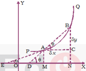
In figure the curve PQ represents the function y = f(x). Let the coordinates of the point A be (x, y) and that of B be \( \left( {x\, + \,\delta x,\,\,y + \delta y} \right) \). Draw suitable perpendiculars as shown in the figure.
\( AC = ON - OM = \left( {x + \delta x} \right) - x = \delta x \) \( BC = BN - CN = \left( {y + \delta y} \right) - y = \delta y \)
\( \frac{{\delta y}} {{\delta x}} = \frac{{BC}} {{AC}} \) = tan\( \theta \), where \( \theta \) is the angle which the line AB makes with the positive direction of x–axis. When \( \delta x \to 0 \), B almost coincides with A, the straight line becomes almost tangent to the curve at A and let \( \alpha \) be the angle made by the tangent with the positive direction of x–axis. This means as \( \delta x \to 0 \), \( \theta \to \alpha \) .
\( \mathop {Lt}\limits_{\delta x \to 0} \frac{{\delta y}} {{\delta x}} = \tan \,\alpha \) or \( \frac{{dy}} {{dx}} = \tan \alpha \)
Hence the differential coefficient at any point gives the slope of the curve at that point.
1. Basic Theorems on Differentiation:
i) The derivative of a constant is zero.
Let y = f(x) = c. Where c is constant.
Then \( \frac{{dy}} {{dx}} = \frac{d} {{dx}}\left( c \right) = 0 \)
Example: Differentiate y = 2a where a is a constant \( \frac{{dy}} {{dx}} = \frac{d} {{dx}}\left( {2a} \right) = 0 \)
ii) The differential coefficient of xn is obtained by decreasing the power of x by unity and multiplying by n.
If y = xn then , where n may be positive or negative.
Example: Differentiate (i) y = x10 and (ii) y = x–2. w.r.t. x
Solution: (i)\( \frac{{dy}} {{dx}} = \frac{d} {{dx}}\left( {x^{10} } \right) = 10x^9 \) . (ii)\( \frac{d} {{dx}}\left( {x^{ - 2} } \right) = - 2x^{ - 2 - 1} = - 2x^{ - 3} \)
iii) The derivative of the product of a constant and a function is equal to the product of the constant and the derivative of the function.
Let u be a function of x and “c” is a constant i.e., y = cu
Then \( \frac{{dy}} {{dx}} = \frac{d} {{dx}}\left( {cu} \right) = c\frac{{du}} {{dx}} \)
Example: Differentiate y = 8x8 w.r.t. x.
Solution: \( \frac{{dy}} {{dx}} = \frac{d} {{dx}}\left( {8x^8 } \right) = 8\frac{d} {{dx}}\left( {x^8 } \right) = 8 \times 8 \times x^{8 - 1} = 64x^7 \)
iv) The derivative of the algebraic sum of two functions is equal to the algebraic sum of the derivatives of the two functions.
Let y = u \( \pm \) v \( \pm \) w \( \pm \).......where u, v, w.....are all functions of x.
Then \( \frac{{dy}} {{dx}} = \frac{d} {{dx}}\left( {u \pm v \pm w \pm ...} \right) = \frac{d} {{dx}}\left( u \right) \pm \frac{d} {{dx}}\left( v \right) \pm \frac{d} {{dx}}\left( w \right) \pm .... \)
Example: Differentiate y = 3x4 + 2x2 – 10x w.r.t. x.
Solution: \( \frac{{dy}} {{dx}} = \frac{d} {{dx}}\left( {3x^4 + 2x^2 - 10x} \right) = \frac{d} {{dx}}\left( {3x^4 } \right) + \frac{d} {{dx}}\left( {2x^2 } \right) - \frac{d} {{dx}}\left( {10x} \right) \)
\( = 4.3.x^{4 - 1} + 2.2.x^{2 - 1} - 10.x^{1 - 1} = 12x^3 + 4x - 10 \)
Rules of differentiation
Product Rule: The differential coefficient of the products of two functions = 1st function × differential coefficient of the 2nd function + 2nd function × differential coefficient of the 1st function.
Let y = u v where u and v are functions of x. Then \( \frac{{dy}} {{dx}} = \frac{d} {{dx}}\left( {uv} \right) = u\frac{{dv}} {{dx}} + v\frac{{du}} {{dx}} \)
Example: Differentiate y = x(x2 – 2x) w.r.t. x.
Solution: Here u = x, v = x2 – 2x\( \frac{{dy}} {{dx}} = \frac{d} {{dx}}\left[ {x\left( {x^2 - 2x} \right)} \right] = x\frac{d} {{dx}}\left( {x^2 - 2x} \right) + \left( {x^2 - 2x} \right)\frac{d} {{dx}}\left( x \right) \) .
\( = x\left( {2x - 2} \right) + \left( {x^2 - 2x} \right) \times 1 = 3x^2 - 4x \)
Quotient Rule: The differential coefficient of quotient of two functions = [2nd function × derivative of the 1st function – 1st function × derivative of 2nd function] divided by the square of the second function.
Let y = u/v where u and v are two functions of x.
Then,\( \frac{{dy}} {{dx}} = \frac{d} {{dx}}\left( {u/v} \right) = \frac{{v\left( {du/dx} \right) - u\left( {dv/dx} \right)}} {{v^2 }} \)
Example: Differentiate y = (x2 + 1)/(x – 1) w.r.t. x.
Solution: Here u = x2 + 1, v = x – 1.
\( \frac{{dy}} {{dx}}\,\,\,\, = \frac{d} {{dx}}\left[ {\left( {x^2 + 1} \right)/\left( {x - 1} \right)} \right] = \frac{{\left( {x - 1} \right)\frac{d} {{dx}}\left( {x^2 + 1} \right) - \left( {x^2 + 1} \right)\frac{d} {{dx}}\left( {x - 1} \right)}} {{\left( {x - 1} \right)^2 }} \)
=\( \frac{{\left( {x - 1} \right) \times 2x - \left( {x^2 + 1} \right) \times 1}} {{\left( {x - 1} \right)^2 }} = \frac{{x^2 - 2x - 1}} {{\left( {x - 1} \right)^2 }} \)
Chain rule or function of a function rule:
Let y = f (u) where y is a function of u and u is a function of x . Then ,
\( \frac{{dy}} {{dx}} = \frac{{dy}} {{du}}.\frac{{du}} {{dx}} \)
Example: Differentiate y = (4x2 – 5x +10)10 w.r.t. x.
Solution: Let 4x2 – 5x + 10 = u. Then y = u10
\( \frac{{dy}} {{du}} = \frac{d} {{du}}\left( {u^{10} } \right) = 10u^9 \)- - - - - - - - - - - - -(1)
\( \frac{{du}} {{dx}} = \frac{d} {{dx}}\left( {4x^2 - 5x + 10} \right) = \left( {8x - 5} \right) \)- -- - - (2)
Now, \( \frac{{dy}} {{dx}} = \frac{{dy}} {{du}}.\frac{{du}} {{dx}} = 10u^9 \times \left( {8x - 5} \right) = 10\left( {4x^2 - 5x + 10} \right)^9 \times \left( {8x - 5} \right) \)
Differentiation of parametric forms:
Let x and y be functions of a parameter \( \theta \) then \( \frac{{dy}} {{dx}} = \frac{{dy/d\theta }} {{dx/d\theta }} \)
Example. Find \( \frac{{dy}} {{dx}} \), Given x = acos3\( \theta \) and y = b sin3\( \theta \)
Solution. \( \frac{{dx}} {{d\theta }} = a.3\cos ^2 \theta \frac{d} {{d\theta }}\left( {\cos \theta } \right) = \)\( 3a\,\cos ^2 \theta \left( { - \sin \,\theta } \right) = - 3a\,\sin \,\theta \,\cos ^2 \,\theta \)- - - - (1)
\( \frac{{dy}} {{d\theta }}\, = \,b.3\sin ^2 \theta .\frac{d} {{d\theta }}\left( {\sin \theta } \right) = 3b\,\sin ^2 \theta .\cos \theta = 3b\,\sin ^2 \theta \,\cos \theta \) - - - - - - - (2)
\( \frac{{dy}} {{dx}} = \frac{{dy/d\theta }} {{dx/d\theta }} = \frac{{3\,b\,\sin ^2 \theta \,\cos \,\theta }} {{ - 3a\,\sin \,\theta \,\cos ^2 \theta }} = \frac{{ - b}} {a}\tan \theta \)
Differential coefficients of Trigonometrical functions
1.\( \frac{d} {{dx}}\left( {\sin x} \right) = \cos \,x \) 2.\( \frac{d} {{dx}}\left( {\cos x} \right) = - \sin \,x \)
3.\( \frac{d} {{dx}}\left( {\tan x} \right) = \sec ^2 \,x \) 4. \( \frac{d} {{dx}}\left( {\cot x} \right) = - co\sec ^2 \,x \)
5. \( \frac{d} {{dx}}\left( {\sec x} \right) = \sec \,x\,\tan \,x \) 6.\( \frac{d} {{dx}}\left( {co\sec x} \right) = - co\sec \,x\,\cot \,x \)
Maxima And Minima: Suppose a quantity y depends on another quantity x in a manner shown in figure. It becomes maximum at x1 and minimum at x2.
At these points the tangent to the curve is parallel to the X – axis and hence its slope is \( \tan \theta = 0 \). But the slope of the curve y(x) equals the rate of change \( \frac{{dy}} {{dx}}. \)
Thus, at a maximum or a minimum, \( \frac{{dy}} {{dx}}. \)
Just before the maximum the slope is positive, at the maximum it is zero and just after the maximum it is negative. Thus, \( \frac{{dy}} {{dx}}. \) decreases at a maximum and hence the rate of change of \( \frac{{dy}} {{dx}} \) is negative at a maximum i.e. \( \frac{d} {{dx}}\left( {\frac{{dy}} {{dx}}} \right) < 0 \) at a maximum. The quantity \( \frac{d} {{dx}}\left( {\frac{{dy}} {{dx}}} \right) \) is the rate of change of the slope. It is written as \( \frac{{d^2 y}} {{dx^2 }} \).
Thus, the condition of a maximum is \( \left. {\begin{array}{*{20}c} {\frac{{dy}} {{dx}} = 0} \\ {\frac{{d^2 y}} {{dx^2 }} < 0} \\ \end{array} } \right] \)– maximum
Similarly, at a minimum the slope changes from negative to positive. The slope increases at such a point and hence \( \frac{d} {{dx}}\left( {\frac{{dy}} {{dx}}} \right) > 0 \).
The condition of a minimum is \( \left. {\begin{array}{*{20}c} {\frac{{dy}} {{dx}} = 0} \\ {\frac{{d^2 y}} {{dx^2 }} > 0} \\ \end{array} } \right] \)– minimum